Equation of Circle in 3D and Snap Tangent

For a time I was on a bit of an AutoCAD like calculation kick and went through some interesting calculations like snap tangent, snap perpendicular, and intersection of a line with a plane. I wanted to take the next step on snap tangent and consider snap tangent to a sphere.

Snap tangent means, start with some point and try to find a point on the destination object (circle, sphere, ellipse, anything) that causes the line segment between the first point and the second point to be tangent to the object selected. My post about snap tangent, showed the result for a circle and worked in 2D. If you get the concept in 2D and are ready to take the concept to 3D for a sphere, you probably recognize without proof that the set of possible points on the sphere which will result in a tangential point, forms a circle. You can pretty much mentally extrapolate from the following picture which a repeat from the previous post.

Fig. 1 - Can you imagine the snap tangent circle on this if we allow the figure to represent a sphere? The snap tangent circle has center \(E\) and radius \(a\).

I will not repeat the method of calculation from the previous post but will simply observe that we can produce the values \(E\) and \(a\), which are the center and radius of the snap tangent circle. We add to this the normal of this circle, \(N = A - C\), and then normalize \(N\).

So, now we need a way to describe this circle which is not too onerous. A parametric vector equation is the simplest expression of it. We take our inspiration from the classic representation of circles in parametric form, which is
\[ p(\theta) = (x(\theta), y(\theta)) \] \[ x(\theta) = r \cos{\theta} \] \[ y(\theta) = r \sin{\theta}. \]
We have a normal from which to work from, but we need to have an entire coordinate system to work with. The classic parametric equations have everything in a neat coordinate system, but to describe a circle that's oriented any which way, we need to cook up a coordinate system to describe it with. Observe a change to the foregoing presentation that we can make:
\[ p(\theta) = r \cos{\theta} (1, 0) + r \sin{\theta} (0, 1) = r \cos{\theta} \vec{x} + r \sin{\theta} \vec{y}\]
The normal vector we have is basically the z-axis of the impromptu coordinate system we require, but we don't have a natural x-axis or y-axis. The trouble is there are an infinite number of x-axes that we could choose, we just need something perpendicular to \(N = (n_x, n_y, n_z).\) So, let's just pick one. If I take the cross product between \(N\) and any other vector that isn't parallel to \(N\), I will obtain a value which is perpendicular to \(N\) and it can serve as my impromptu x-axis. To ensure I don't have a vector which is close to the direction of \(N\), I will grab the basis vector, which is the most "out of line" with the direction of \(N\). So, for example (F# style),

        let b = if abs(normal.[0]) <= abs(normal.[1]) then    
                    if abs(normal.[0]) <= abs(normal.[2]) then
                        DenseVector([| 1.0; 0.0; 0.0 |])
                    else
                        DenseVector([| 0.0; 0.0; 1.0 |])
                else
                    if abs(normal.[1]) <= abs(normal.[2]) then
                        DenseVector([| 0.0; 1.0; 0.0 |])
                    else
                        DenseVector([| 0.0; 0.0; 1.0 |])

In this case, I have 

\[\vec{x} = b \times N\] \[\vec{y} = N \times \vec{x}.\]

Using this impromptu coordinate system, I can express an arbitrary circle in parametric form, having center \(C\) and radius \(r\) as

\[ p(\theta) = C + \vec{x} r \cos{\theta} + \vec{y} r \sin{\theta}.\]

Thus, our snap tangent circle is given from above as 

\[ p(\theta) = E + \vec{x} a \cos{\theta} + \vec{y} a \sin{\theta},\]

where we would use \(N = A - C\) (normalized) to be the beginning of our coordinate system.

Packing Spheres into a Cube

In this post I compare three different alignment strategies for putting spheres into a cube. Our main variable will be \(n\), the ratio of cube side to sphere diameter. The question is, how many spheres can we get into the cube? We denote the number of spheres as \(S\).

Matrix Alignment

The simplest alignment of spheres to think about is a matrix alignment, or row, column, layer. If \(n=10\), then we can fit 1000 spheres into the cube this way. Or, in general, \(S=n^3\).

Fig. 1. Matrix alignment.

One way to summarize this alignment is that each sphere belongs to its own circumscribing cube and none of these circumscribing cubes overlap each other. For small values of \(n\), this arrangement is optimal.

Square Base Pyramid Alignment

An improvement to \(S\), for larger values of \(n\) is had by making the alignment of subsequent layers offset. Start with a layer in a square arrangement (\(n\) by \(n\)). If you look down on this first layer, it's awfully tempting to nestle the next layer of spheres in the depressions between the spheres. We will make better use of the interior space, although we won't make as good a use of the space near the edges. But if we can get enough extra layers in to make up for the losses near the outside, that would carry the day.

Fig. 2. A few red dots show where we're thinking of putting the next layer of spheres. We won't fit as many on this layer, but the second layer isn't as far removed from the first.

In the matrix alignment, consecutive layers were all a distance of 1 unit between layers (center to center). With this current alignment, we need to know the distance between layers. We need to consider a group of four spheres as a base and another sphere nestled on top and find the vertical distance from the center of the four base spheres to the center of the top sphere. (Implicitly, the flat surface the four base spheres are resting on constitute horizontal. Vertical is perpendicular to that.)

Fig. 3. Top view of a square base pyramid packing arrangement.

We can see from Fig. 3., that line segment ab is  of length \(\sqrt{2}\). We take a section parallel to this line segment, shown in Fig. 4.

Fig. 4. We recognize a 45°-45°-90° triangle, abc.

We can calculate the vertical distance between layers, line segment cd, as \(\sqrt{2}/2 \approx 0.7071\dots\). Note that the spheres in this second layer are in basically the same configuration as the bottom layer. We can see this will be the case because the top sphere in Fig. 3., has its outer circumference pass across the point where the lower spheres meet. So adjacent spheres in the second layer will be in contact. And, further, second layer spheres will follow the rectangular pattern of depressions in the bottom layer which are spaced apart the same as the centers of the spheres in the bottom layer. So we will end up with the same organization of spheres in the second layer as the bottom layer, just one fewer row and one fewer column.
We can now calculate the number of spheres that will fit in a cube using this alignment as

$$S = n^2 \lambda_1 + (n-1)^2 \lambda_2,$$

where \(\lambda_1\) is the number of full layers and \(\lambda_2\) is the number of "nestled" layers. (The third layer, which is indeed "nestled" into the second layer is also returned to the configuration of the first layer and so I refer to it as a full layer instead. The cycle repeats.) To find \(\lambda_1\) and \(\lambda_2\), we first find the total layers, \(\lambda\) as

$$\lambda = \left \lfloor{\frac{n-1}{\sqrt{2}/2}}\right \rfloor+1$$

The rationale for this formula is: find how many spaces between layers there are and compensate for the difference between layers and spaces. Imagine a layer at the very bottom and a layer at the very top (regardless of configuration). The layer at the bottom, we get for free and is the 1 term in the formula. (The top layer may or may not be tight with the top when we're done but hold it up there for now.) The distance from the center of the bottom layer to the center of the top layer is \(n-1\). The number of times we can fit our spacing interval into this number (completely), is the number of additional layers we can fit in. (Additional to the bottom layer, the top layer is the last of the layers we just found room for in the \(n-1\), or, technically, \(n-1/2\), er, whatever, do some examples.)

The break down between \(\lambda_1\) and \(\lambda_2\) will not be exactly even, with \(\lambda_1\) having one more if \(\lambda\) is odd. We can show this neatly using the ceiling operator 

$$\lambda_1 = \left \lceil{\lambda/2}\right \rceil$$

$$\lambda_2 = \lambda - \lambda_1$$

As early as \(n=4\) we get \(S=66\), which is better than the matrix arrangement by 2 spheres. I modeled this to make sure I didn't let an off by one error sneak into my formula (see Fig. 5.).

Fig. 5. Somewhat surprisingly, rearrangement of spheres (relative to matrix alignment) produces gains in volume coverage even at \(n=4\).

Here it is in Maxima:

SquareBasePacking(n) := block([lambda_1, lambda_2, lambda], lambda: floor((n-1)/(sqrt(2)/2))+1, lambda_1: ceiling(lambda/2), lambda_2: lambda - lambda_1, n^2 * lambda_1 + (n-1)^2 * lambda_2);

Tetrahedral Alignment

Another rearrangement is similar to a honeycomb. A honeycomb is an arrangement of hexagons that meet perfectly at their edges. Pictures of this are readily available online. This Wikipedia article suffices. Imagine putting a circle or a sphere in each of these honeycomb cells. The will produce a single layer which is more compact, although it will push the distance between layers apart. 

So, what do we need to know to make a formula for this one?

1. Find the distance between successive layers.
2. Formula for the number of layers.
3. Formula for the number of spheres in each layer.
1. This depends on knowing the range of layer configurations (we will only have two different layer configurations).
4. Some assembly required.

This is the same procedure we followed already for the square based pyramid alignment, but we are being more explicit about the steps.

Fig. 6. We need to find the distance of line segment ad.

We recognize we have an equilateral triangle and so we can identify a 30°-60°-90° triangle on each half of altitude ab. We have drawn all of the angle bisectors for this triangle which meet at a common point (commonly known property for triangles). We can recognize/calculate the length of bd as \(\frac{1}{2\sqrt{3}}\). We can then calculate the length of ad as \(\frac{\sqrt{3}}{2} - \frac{1}{2\sqrt{3}} = 1/\sqrt{3}\). From the Pythagorean theorem, we have a length for cd of \(\sqrt{2/3}\).
The number of spheres in the first layer will require us to use the distance for ab. We now need to find the number of rows in the bottom layer. We have
$$L_1=n \rho_1 + (n-1) \rho_2,$$
where \(\rho_1\) and \(\rho_2\) are the number of each kind of row in the layer and \(L_1\) is the number of spheres in the first layer. Since rows are spaced by \(\sqrt{3}/2\), we have a number of rows, \(\rho\), of
$$\rho = \left \lfloor{\frac{n-1}{\sqrt{3}/2}}\right \rfloor+1$$
and \(\rho_1\) and \(\rho_2\) can be broken out similar to our \(\lambda\)'s earlier.
$$\rho_1 = \left \lceil{\frac{\rho}{2}}\right \rceil$$
$$\rho_2 = \rho - \rho_1.$$

Fig. 7. We're looking for the distance of line segment cd which can be found using ac and ad.

Now, there is a little matter of how nicely (or not) the second layer will behave for us. It is noteworthy that we are not able to put a sphere into every depression. We skip entire rows of depressions. (The Wikipedia article on sphere packing referred to these locations as the "sixth sphere".) These skipped locations may play mind games on you as you imagine going to the third layer. Nevertheless, the third layer can be made identical to the first, which is what I do here.

Fig. 8. The first layer is blue. The second layer is red. Are we going to have trouble with you Mr. Hedral?

There's a couple of things that happen on the second layer. First, instead of starting with a row of size \(n\), we start with a row of size \(n-1\). The second issue is that we may not get as many total rows in. We could do the same formula for rows again but now accounting for the fact that we have lost an additional \(\frac{1}{2\sqrt{3}}\) before we start. However, we can reduce this to a question of "do we lose a row or not?" The total distance covered by the rows, \(R\), for the bottom layer is
$$R = (\rho-1) \frac{\sqrt{3}}{2} + 1$$
If \(n-R\ge\frac{1}{2\sqrt{3}}\), then we have the same number of total rows. Otherwise, we have one less row. We let \(r_L\) represent the number of rows lost in the second layer, which will either be 0 or 1. Noting that the order of the rows is now \(n-1\) followed by \(n\), we can give an expression for the number of spheres, \(L_2\), in our second layer now.
$$L_2 = (n-1)(\rho_1 - r_L) + n\rho_2$$
We have a very similar formula for the total number of spheres in the box.
$$S = L_1\lambda_1 + L_2\lambda_2,$$
where
$$\lambda_1 = \left \lceil{\frac{\lambda}{2}}\right \rceil$$
$$\lambda_2 = \lambda - \lambda_1,$$
where
$$\lambda = \left \lfloor{\frac{n-1}{\sqrt{2/3}}}\right \rfloor+1.$$
My Maxima function for this is
TetrahedralPacking(n) := block( [lambda_1, lambda_2, lambda, rho_1, rho_2, rho, r_L, L_1, L_2, R], rho: floor((n-1)/(sqrt(3)/2))+1, rho_1: ceiling(rho/2), rho_2: rho - rho_1, L_1: n*rho_1 + (n-1)*rho_2, R: (rho-1) * sqrt(3)/2 + 1, r_L: if n - R >= 1/(2*sqrt(3)) then 0 else 1, L_2: (n-1)*(rho_1 - r_L) + n*rho_2, lambda: floor((n-1)/sqrt(2/3))+1, lambda_1: ceiling(lambda/2), lambda_2: lambda - lambda_1, L_1 * lambda_1 + L_2 * lambda_2);

Comparison Between Methods

It isn't too hard to tell that one of the two second approaches is going to produce better results than the first after some value of \(n\) (Fig. 9.). What is more surprising is that our latter two alignments stay neck and neck up into very high values of \(n\). If we divide them by the volume of the containing cube, both appear to be a round about way to arrive at the square root of 2! (Fig. 10.)

Fig. 9. Both of the latter approaches give much better packing densities than the matrix alignment.

Fig. 10. Square base packing in blue, tetrahedral packing in red, both divided by total volume (# of spheres/unit volume). Unclear if there is a distinct winner and we seem to be getting closer to \(\sqrt{2}\).

Let's see which one wins more often for positive integer values of \(n\) in Maxima.

So, there's no run away winner, but if you're a betting man, bet on square base pyramid packing out of the available choices in this post. Regardless, it appears that both of these packing arrangements approach optimal packing (see Sphere packing). My density calculation (allowing the \(\sqrt{2}\) conjecture) for volume coverage comes out to

Gauss, old boy, seems to have approved of this number.

Skew Cut Profiles

I recently was surprised (anew) at what happens when you cut a prism which has a uniform cross-section with a plane which is not orthogonal to the length of the prism. Especially if the plane must be described in terms of two angles. A cross-section through a square prism is (by definition) a square. If you make your cut at an angle, you will get a rectangle if you have a simple angle cut. But if you make your cut not only a miter, but also a bevel you end up with a parallelogram.

The simplest way to visualize this is to imagine a plane that intercepts the prism at a single edge first and has its steepest slope in the direction of the opposite edge:

The resulting section when viewed in the intersecting plane would be something like this:

where the blue square is the cross-section, the red parallelogram is the intersection of the above described plane through the square prism when viewed in that plane. (A few thought experiments of your own will probably serve you better than any further illustration of this phenomenon I could drum up at the moment.)

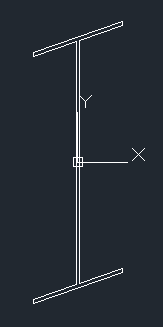
It is interesting to see the result in an I-beam shape if you use a 45° miter and 45° bevel:



As a matter of where this observation fits into mathematics generally, this is a projective or affine transformation. Such transformations preserve straight lines but they do not, in general, preserve right angles.

Aside: Convex Hulls

The fact that they preserve straight lines is a boon to the would-be-writer of a convex hull algorithm in an arbitrary plane since you can project the 3D coordinates onto a simple 2D plane and use the 2D algorithm (being careful to preserve or restore the other coordinate at the end). If you do so, you should probably choose which set of 2 coordinates to use for the algorithm, based on the direction of the plane. For example, if the normal of the plane has a larger z-coordinate than x- or y-coordinates, then the (x,y) pairs are best to use for the information to run the 2D convex hull algorithm on. There are two reasons to be picky about this:

1. If the points fed to the routine are in thy yz-plane, you will get incorrect results (if you assumed the (x,y) coordinates should always be used).
2. It may reduce the effect of rounding errors in the calculations (in terms of deciding whether points "near the line" of the hull are inside or part of the hull).

(I have lost the original code I used for this post, so I omit references to it now.)

See the Maxima project for download information for Maxima.

The Un-Pyramid

In previous posts I've discussed truncated pyramids and irregular triangular prisms, but I hadn't at that time thought to consider a "really irregular triangular prism" before.  I was searching on the general notions of these topics on the internet to see what people were thinking about with respect to them and found someone had something different in mind:  A 5 sided solid with a non-constant triangular cross-section and no faces (guaranteed) parallel with each other.

The first thing to note about this shape is the characterization of the faces.  The two "ends" are triangular faces. There are three quadrilateral faces which form the boundaries of the non-constant triangular cross-section. The three edges shared by the quadrilateral faces are not parallel with each other and the quadrilaterals could be completely irregular. Here is a quick video of a Sketchup model of just such a shape:


The Un-Pyramid from Darren Irvine on Vimeo.

Since the consecutive pairs of "side" edges are part of a quadrilateral (they are proper "faces"—no twists), they are certainly coplanar. In a previous post, I demonstrated that two parallel faces with edges joining corresponding vertices with consecutive edges being coplanar, the parallel faces are necessarily similar. I also demonstrated (Proposition 4) that the projected side edges intersect at a common point, which we may call the apex.

The un-pyramid does not have the two parallel faces that formed the starting point in that post. However, it does have the consecutive coplanar edges. And although we have not been given a "top" face parallel with the bottom, we can certainly make one. We establish a cutting plane through the closest vertex (or vertices—there could be two at the same level) of the "top" face which is parallel with the larger "bottom" face. (We can turn the un-pyramid around to make the names fit if it comes to us upside down or sideways.) Now we can be sure that the side edges can be projected to a common apex as per 3D Analogue to the Trapezoid (part 3).

Fig. 1.  A really irregular triangular pyramid? Hmm...

Calculating the volume of this shape requires a bit of calculation just to figure out how to break it up into pieces. If you want to program a solution to this problem, you are probably going to take in A₁, B₁, C₁, A₂, B₂, and C₂ as the parameters. To verify you have valid data establish that:

• A₁A₂ is coplanar with B₁B₂
• B₁B₂ is coplanar with C₁C₂
• C₁C₂ is coplanar with A₁A₂
• Also, make sure these same edges don't intersect each other (meaning the lines projected through them should intersect outside of the boundaries of the line segments).

You also need to determine whether the apex is closer to A₁B₁C₁ or A₂B₂C₂. Then reorder or relabel the end faces as necessary. The face further away is the base (say ₁). Now determine which of the top vertices is closest to the base and establish a cutting plane through it, parallel to the base.

(Hint: It will be convenient to reorder or relabel your points so that A₂ is the closest point, B₂ next, and C₂ furthest; this avoids polluting your code with cases. Don't forget to reorder the points in the base. You may have a job making the relabeling of previous calculation results work properly. Making clear code that does minimal recalculations is probably the most challenging aspect of this problem if treated as a programming challenge.)

Now we can calculate the volume as a sum of two volumes:

1. Frustum of a (slanted) pyramid with base A₁B₁C₁ and top A₂BC.
• For the overall formula, see 3D Analogue to the Trapezoid (part 2)
• To find the areas of the top and bottom, use the cross-product method (see Area of Triangle Given Coordinates)
• To find the height, find the component of vector (A₂ – A₁) perpendicular to the base (also used in Volume of a Tetrahedron)
2. Slanted pyramid with base BB₂C₂C and apex A₂
• Find the area of the base
• watch out for B = B₂ and C = C₂ which changes the shape of the base
• If both are true, then you've dodged the bullet—there's no volume to worry about.
• If B = B₂, then either it is at the same level as C₂ or the same level as A₂. But in either case, you have a triangular base.
• Very possibly neither of these will be true. Break the quadrilateral up into two triangles using the diagonal of your choice.
• Find the height of the pyramid using the component method as for finding the height of the first volume.

But, what should we call it?

1. triangular un-pyramid
2. really irregular triangular prism
3. skew-cut slanted triangular pyramid
• alternatively, skew-cut slanted pyramid with triangular base

I guess I like 1) for the advertizing, 2) for the baffling rhetorical effect, and 3) for half a hope of conveying what the shape really is.

Find the Intersection of a Plane with a Line

We can represent a plane with four numbers, the coefficients of the general equation of a plane, as ax + by + cz + d = 0.  For convenience, we can represent this also as

where n = (a, b, c) and r = (x, y, z) is a point on the plane.

We take a line through two points, A and B, in vector form as

        L(t) = A + (B–A)t

We want to find the intersection of the line with the plane.  That is, we need f, such that

Then,

And so

The desired point is L(f), since it on the plane and on the line.

Notice that the calculation of f requires only the evaluation of the general equation of the plane using A and B as the points. The results will not be zero unless A and B are on the plane, in which case we would already have the result. If the line is parallel with the plane, then the denominator will be zero giving an indeterminate result. This fits with the geometric interpretation of the plane evaluation. The point of the last step in our derivation is that it simplifies the coding of the problem somewhat by reducing it to two plane evaluations. (If you observe carefully, you will see it makes the difference not of two additions but only of one.)

Evaluating the equation of a plane using a point not on the plane gives a result which is proportional to the distance between the planes. If the normal vector (n = (a, b, c)), has a magnitude of 1, then it yields the distance. However, in the formula we have derived, we have not depended on the equation of the plane being normalized. The constant of proportionality in the numerator cancels with itself in the denominator (I mean "behind the scenes" or if you derived it using a different approach) to produce the simple result for f above.

The idea for this solution came from initially viewing it as a linear interpolation problem, which, of course, it is. Similar triangles also are an acceptable approach the problem, though it may be more difficult to deal with the signs. The above derivation deals with sign transparently.

Volume of a Tetrahedon

In this article I give a rough outline of a derivation of the volume formula for a tetrahedron, given its four vertices.

Any set of three points in 3D are co-planar. If they are not co-linear, then they uniquely define a plane. They also uniquely define a triangle. With polygons of more than three sides/vertices, you need to specify which edges are drawn and which are not.  In a program, you might imply the edges according to the ordering of the points, but the order then is a means of indicating which edges to draw. You could not simply draw all of the possible edges and get a polygon, generally. But with a triangle, you take every pairing of points and draw an edge between them.

If you add a fourth point which is not in the same plane, you now have a tetrahedron (tretra = four)—a four sided polyhedron which is uniquely defined by four points. As in the case of the triangle, you draw an edge between every pairing of points. The number of combinations of 2 points is    

and so there are 6 edges.

A tetrahedron is a special case of a slanted pyramid. The same volume formula applies, namely,
                                                          
In order to use the formula, we must pick a face to serve as the base.  We choose the face with vertices P₁, P₂, and P₃, in the above illustration. (It doesn't matter which ones as long as you're consistent.)  We need to calculate the area of the base and find the height of the pyramid. The height is the distance from P₄ to the plane defined by the base points (the measure is taken perpendicular to the plane).

First we find the area. A well known formula for finding the area of a triangle given the length of two sides, say a and b, and the included angle, say θ,  is      

(With some minor trig you can figure this out, but if you just want to see it proved, see Area of Triangles Without Right Angles [1].) The cross-product comes in handy here since

where v and u are vectors and θ is the included angle. Thus, the area is

To find the distance from P₄ to the base plane, we first find the plane. The equation of a plane can be expressed in terms of a normal vector and any point on the plane. The normal vector for our plane is

and the equation of the plane is

(This is a 3D analogue to the point-slope form of the equation of a line, albeit, it also resembles the general form.)

The height from the plane to P₄ is the component of the vector (P₄ – P₁) which is in the direction of the normal vector, namely ([2], p. 679),

This leads to the volume formula

Sources:

1. Math is Fun, Area of Triangles Without Right Angles, http://www.mathsisfun.com/algebra/trig-area-triangle-without-right-angle.html
2. Stewart, J., Calculus: Early Transcendentals, 3rd Ed., Brooks/Cole Publishing Company, 1995

Rotation of Planar Regions: Polyhedron in AutoCAD

In a previous post about the angle between intersecting planes, I noted the importance of measuring that angle perpendicular to the line of intersection.  Now I want to apply a similar notion to the rotation of planar regions.  In CAD programs that support solid and surface modelling, it is common to support planar regions. These programs do much more complicated things as well, of course, but they will certainly allow you to make, say, a hexagonal region.  A hexagonal region is not only the outline of the hexagon, but the area enclosed by that outline, all of which lies within the same plane as the outline.  Making a planar region in AutoCAD is straightforward:

1. Change to one of the 3D workspaces.
2. Create any closed sequence of line work (sometimes called a closed path), all of which should be coplanar.  (While you can create a closed path that is not coplanar, it won't suit our purpose here and you can't make it into a region.)
3. Type Region, select the line work and press .
4. To see the region, change the visual style as necessary:
1. Click the View tab.
2. Click the Visual Styles button on the Palettes pane.
3. In the Visual Styles Manager (which should pop up) choose a style that shows the faces (if/when that is desirable).  I'm partial to Shaded with edges, but other styles may be suitable.
1. Notice also the settings under Face Settings that can affect the way the faces appear (or not appear).

But I don't just want to make planar regions, we want to do something with them.  I want to rotate them about a line of intersection/adjacency and make multiple regions "fit" together.  I'm going to make, well, you'll see...(at the end of the video in this post)...

Description of the Problem

Suppose we are given three planar regions A, B, and C, such that A is adjacent to B and B is adjacent to C, with all of the regions being initially co-planar with each other.  We want to rotate A and C about their "line of adjacency" with B so that A and C are adjacent to each other.

Informally, we might say that A and C are the box flaps and B is the base.  You may intuit the analogy I'm making.  We are pretending we have a sheet of cardboard cut out in an unusual shape with two creases in it which will serve as the fold lines – our lines of adjacency.  Note also that the proximal lines of A and C (the ones we want to be coincident) need not be of equal length to do the kind of folding/rotating we want to do, but if they are not equal we may not get the result we desire.

We are currently looking at our box flaps in plan view.  Suppose we continue observing in plan view and fold the box flaps (about B).  B is unchanged in appearance but A and C appear "squished" in one direction.  Or, another way to think of it, every point on A will appear to move perpendicularly toward its line of adjacency with B.  Likewise for C.  Thus,

If for some reason the proximal lines of A and C were not of equal length (as they are above), for purposes of our construction, we would need to establish points of equal distance from their common vertex.  A circle centered on their common vertex would do nicely.  In AutoCAD we can work in 3D to do this rotation, but first let's consider how we would do this in 2D.  This will be informative as to how to proceed in 3D.

First observe how the arrows at the end of the proximal lines of A and C cross each other.  These arrows are in plan view with z = 0, but the point where these arrows intersect gives us the xy-coordinates of the point where the non-common vertices of the proximal lines will meet.  (If that doesn't make sense, just go with the picture.)  Now to make our 2D plan view work, we've got to do some single axis scaling.  Here's what we're looking at:

We need to scale region A along the y-axis by a factor of A₂/A₁ and scale C along an axis perpendicular to the line of adjacency with B by a factor of C₂/C₁.  Since we are working with only a small number of points here, we can simply draw lines of lengths A₃ and C₃ and scale them as needed.  We move and copy the lines as necessary so that we can move the vertices of the polygons to their new positions based on the newly scaled lines.  (To scale A in the y direction you could turn A into a block and scale the y-axis as desired.  To scale C you could use the "block"  and scale method too, but you'd have to adjust your UCS line up with the line adjacent to B – use the ucs command with the OBject option and click the line you want to line up with.)  Here's the scaled result:

I used the scale command with the reference option so that I didn't have to do the indicated math myself, but AutoCAD did in fact compute A₃(A₂/A₁) and likewise for C.  (Incidentally, this doesn't work so nice with regions, though it works fine with polylines; it's a simple matter of moving vertices along a line perpendicular to the line of adjacency.)  As for making the other views work for you in 2D – you're on your own, because right now I'm posting how to do this in AutoCAD (full version).

Rotating Planar Regions to Make a Polyhedron in AutoCAD


Making of a Polyhedron in AutoCAD from Darren Irvine on Vimeo.

3D Analogue to the Trapezoid (part 3)

Suppose we have two parallel polygonal faces with a non-zero distance between such that, for some pairing of vertices, every consecutive pair of edges connecting the paired vertices are coplanar. It follows that the faces joining the two given parallel polygonal faces are quadrilaterals.  At first, it might not appear that this is a sufficient condition to assert that the shape thus described is a frustum of a slanted pyramid.  In this post I proceed to prove that it is.  For the volume formula of a frustum of a pyramid (slanted or otherwise), see this previous post of mine.

I term the parallel polygonal faces the end faces and the other faces as the side faces.

Proposition 1 (Transitivity of Parallel Lines).

1. Let P be a plane and L a line parallel with P. Every line parallel with L is also parallel with P.
2. Let L, M, N be lines. Then, if L is parallel with M and M with N, then L is parallel with N.

Proposition 2. The corresponding edges of the polygons are parallel with each other.

Fig. 1. Partial drawing of  two parallel planes.  AC is the "bottom edge" and BD is the "top edge".  AB and CD are "side edges".  Consecutive side edges are coplanar with each other.

Proof: Assume without limitation that the faces are parallel with the horizontal plane. Since the faces are parallel, the edges do not change in proximity vertically. Consider any two consecutive edges AB and CD joining the two end faces with corresponding vertices A with B and C with D. Draw line EF with E on line AC (edge of bottom face) and F on BD (edge of top face; extend BD as necessary) such that EF is perpendicular to AC. EF is coincident with the plane of quadrilateral ABDC and so is coplanar with all of its edges.

Fig. 2. We show the construction of B'D' as a line which is coincident with BD, but this is not given as a condition in the construction. That is to be proved. At construction we take neither parallelness nor coincidence with BD for granted. Because it is the same distance from AC as the point F, however, we do know there is at least an intersection between B'D' and BD at F.

Let B' and D' be points such that AB' and CD' are of length(EF), coincident with the plane of quadrilateral ABDC, and perpendicular to AC. Then AB' and CD' are parallel.

If you want to go crazy with the details to see that B'D' is parallel with AC, see the parenthetical section below. I obviously did want to go crazy. Normal people can skip ahead.

(By side-angle-side, triangle AB'C is congruent with triangle CD'A. Thus,

Also, since the non-right angles of a right triangle sum to 90°,

                                               
Thus, triangles B'AD' and D'CB' are congruent by side-angle-side. Hence,

By alternating interior angles,

Since the angles of a triangle sum to 180°,

Hence, angle B'D'C is a right angle.  By a similar argument, angle D'B'A is a right angle and so quadrilateral AB'D'C is a rectangle and thus B'D' is parallel with AC. Since F is length(EF) away from AC, in the same plane as quadrilateral AB'D'C, on the same side of AC, it is on line B'D'.)

Fig. 3. The shape we are discussing doesn't really look like this, but how do we know it doesn't look like this? How do we know Fig. 2. isn't the one that's wrong? See rest of argument below.

Assume that lines BD and B'D' are not coincident. Both are coincident with a common plane and so are coplanar. Since quadrilateral ABDC is on an angle from horizontal and BD and B'D' are not coincident, there is some point, P, on B'D' which is below BD. But point F is coincident with both BD and B'D'. Since BD is parallel with horizontal (it is part of a polygonal face which is horizontal), and B'D' has at a point on and a point below BD (points F and P, respectively), B'D' is not parallel with the horizontal plane. But, since AC is parallel with the horizontal plane, the parallel line B'D' must be parallel with the horizontal plane (Proposition 1), which is a contradiction. Thus our (limiting) assumption is wrong and lines BD and B'D' are coincident. It follows that BD is parallel with AC.■

Corollary 1. The walls of the prism are trapezoidal.

Proof: The corresponding edges of the end faces are parallel.■

Corollary 2. Every cross-section of the prism, parallel with the end faces, has corresponding edges parallel with the end faces.

Proof: Fix any cross-section parallel with the end faces and observe that the side edges are intersected by this cross-section so as to produce a polygonal face, whose vertices and edges correspond with the bottom face in the same way the top face did in the proof of Proposition 2. The same argument, therefore, applies.■

Proposition 3. The top and bottom faces are similar shapes.

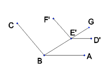
Proof: It suffices to show that the interior angles at each pair of corresponding vertices are equal. Let A, B, and C be consecutive vertices of the bottom polygon and D, E, and F be the corresponding vertices of the top polygon, respectively. By Proposition 2, DE is parallel with AB and EF is parallel with BC. There exists vertices D’, E’, and F’ which are translated vertically from the top polygonal face down to the plane of the bottom polygon. By this we obtain lines D’E’ and E’F’, in the plane of the bottom polygon which are parallel with DE and EF, respectively. By Proposition 1, D’E’ is parallel with AB and E’F’ is parallel with BC. Draw a line through B and E’ to some point beyond E’, say, G (see Figure 1).

Figure 1. AB || D’E’ and BC || E’F’.

Then we have corresponding angles ABE' = D'E'G and CBE' = F'E'G. Thus, ABC = D'E'F'. We take for granted that the translation of DEF to D’E’F’ did not alter the angle between the lines and so we have our result.■

Corollary 3. The cross-section taken parallel with the end faces is everywhere similar to the ends.

Proof: By observing that the parallel cross-section intersects the trapezoidal walls of the prism so as to produce lines which are parallel to the base and top (Corollary 2), the argument applied for Proposition 3 applies here as well.■

Proposition 4.  The lines extended from the side edges intersect at a common point (the apex).

Proof:  Consider three consecutive vertices on the base A, B, and C, and corresponding vertices D, E, and F on an arbitrary parallel cutting plane parallel with ABC. By corollary 3,

Since AD and BE are coplanar, they intersect at some point P. Similarly, BE and CF intersect at some point Q. Assume that P ≠ Q. Take a section parallel to the base through P and label the vertices of the section which correspond to A, B, and C as D, E, and F and observe that the above proportion equation still follows from corollary 3. Also, D = E = P and so line segment DE = 0. However, since P ≠ Q, line segment EF ≠ 0, which contradicts the proportion above. Therefore, our assumption that P ≠ Q is wrong and we have P = Q. By the principle of mathematical induction, the proposition follows.  [Finding P is (i) 2 in S and establishing P = Q is (ii) the inductive step. 1 in S is either automatic or ill-defined I suppose, but irrelevant anyway.]■

The shape we have considered in this post is a frustum of a (possibly slanted) pyramid by proposition 4.

We conclude by noting that the argument for determining the volume of the frustum of a pyramid does not impose a condition that requires the top face to be centered over the bottom face. A slant does not alter the argument and therefore the result is the same. Note, of course, that the height must be measured perpendicularly to the end faces. It should be noted that we have not dealt in this post with the relationship between the cross-sectional area and the height, which relationship is needed in order to establish the volume formula.

Such proof involves 1) similar triangles, using the height of the apex as a reference, and 2) the relationship between linear dimensions and the area(s) they pertain to. Assurance of the existence of a proper apex is the critical component addressed in this post.

Thanks to one of my readers for the question at the end of a previous post that led to this post.

Unfolded Approximation to a Hemisphere

The animated GIF featured below are a sort of slide show which give increasing levels of precision in polyhedral approximations to a hemisphere. The SVG one works properly in Google Chrome, but it may not work in all browsers. In theory, you could print these out, cut along the outline, and fold along the internal lines and you would have a polyhedral approximation to a sphere—if you use a lot of tape and your very best dexterity. More precisely, all of the corners would be coincident with the hemisphere being approximated. Notice that as the number of fold lines (latitudinal-ish lines) increases, for a given number of segments (longitudinal-ish divisions) the extent of the unfolded approximation approaches the grey line, which (probably) represents the limiting extent of these approximations. Specifically, this circle has radius of πr/2 or one fourth the circumference of the approximated sphere.

I wrote the code which generates this sequence of pictures in Maxima, a computer algebra system. The code is below and you can modify the range variable near the end to change the level of precision in the resulting pictures. The pattern for each range item is

[number of segments, [starting latitude divisions, ending latitude divisions]]

The "segments" are longitudinal segments like an orange. The latitude divisions are the number of latitude divisions in each of the segments.

load(draw)$ ExplodedHemiSphereLine(radius, deltaAlpha, theta) := block([line,vc,alpha,xpnm1,ypn,upperThresh,x,y,w,xpn], line: Polyline([0,0]), vc: radius*sqrt(2*(1-cos(deltaAlpha))), alpha: deltaAlpha, xpnm1: 0, ypn: 0, upperThresh: 3.14159265358979/2 + deltaAlpha/2, while alpha <= upperThresh do ( x: radius*sin(alpha), y: radius*cos(alpha), w: x*sqrt(2*(1-cos(theta))), xpn: w/2, dvn: sqrt(vc^2 - (xpn - xpnm1)^2), ypn: ypn + dvn, xpnm1: xpn, line: append(line, Polyline([xpn, ypn])), alpha: alpha + deltaAlpha ), return(line) )$ Reflect(points) := map(lambda([p],[-p[1],p[2]]), points)$ MakePrimaryLines(polyLine) := block([reflection,lis], reflection: Reflect(polyLine), lis: [polyLine, reflection], for i: 2 thru length(polyLine) do ( lis: append(lis, [Line(part(polyLine,i),part(reflection,i))]) ), return(lis) )$ RotatePoint(point, rotationVector) := [point[1]*rotationVector[1] - point[2]*rotationVector[2], point[1]*rotationVector[2] + point[2]*rotationVector[1]]; RotateLine(line, rotationVector) := block([p,res], res: part(line,0)(), for p in line do ( res: append(res, part(line, 0)(RotatePoint(p, rotationVector))) ), return(res) )$ RoundTheWorld(line, rotationVector, Ns) := block([lines,i], lines: [line], for i: 2 thru Ns do ( lines: append(lines, [RotateLine(lines[i-1], rotationVector)]) ), return(lines) )$ ExplodedHemiSphere(radius, Na, Ns) := block([deltaAlpha,theta,line,baseLines,allLines,rotationVector,obj], deltaAlpha: 3.14159265358979/(2*Na), theta: 2*3.14159265358979/Ns, line: ExplodedHemiSphereLine(radius, deltaAlpha, theta), baseLines: MakePrimaryLines(line), allLines: [], rotationVector: [cos(theta), sin(theta)], for obj in baseLines do ( allLines: append(allLines, RoundTheWorld(obj, rotationVector, Ns)) ), return(allLines) )$ FindMinMax(LineObjects, index) := block([min,max,p,obj], min: part(LineObjects[1],1)[index], max: min, for obj in LineObjects do ( for p in obj do ( if p[index] < min then ( min: p[index] ) else if p[index] > max then ( max: p[index] ) ) ), return([min, max]) )$ MakeScene(LineObjects) := block([res], res: gr2d(color = grey, fill_color = white, points_joined = true, point_type = none, axis_top = false, axis_bottom = false, axis_left = false, axis_right = false, xtics = none, ytics = none, ellipse(0,0,float(%pi/2),float(%pi/2),0,360), color = black), for obj in LineObjects do ( if part(obj, 0) = Line then ( res: append(res,gr2d(points([[part(obj,1)[1], part(obj,1)[2]], [part(obj,2)[1], part(obj,2)[2]]]))) ) else if part(obj, 0) = Polyline then ( res: append(res,gr2d(points(makelist([part(obj,i)[1],part(obj,i)[2]],i,1,length(obj))))) ) ), res )$ /* main */ ranges: [[3, [1, 3]], [4, [1, 4]],[5,[1,5]],[6,[1,6]],[7,[1,7]],[8,[1,8]],[9,[1,9]],[10,[1,10]],[11,[1,11]],[12,[1,12]],[13,[1,13]],[14,[1,14]],[15,[1,15]],[16,[1,16]],[17,[1,17]]]$ exp_ranges: map(lambda([u],makelist([1,i,u[1]],i,u[2][1],u[2][2])),ranges)$ ranges: []$ for i: 1 thru length(exp_ranges) do ranges: append(ranges,exp_ranges[i]); draw( delay = 100, dimensions = [500,500], file_name = "C:/Users/whateverpath/whatever", terminal = 'animated_gif, map(lambda([u],MakeScene(ExplodedHemiSphere(u[1],u[2],u[3]))),ranges) )$

Angle Between Intersecting Planes

In a practical sense, there are a few different ways that you can go about determining the angle between two planes.  But before we get to specific methods and tools, let's try to lay the ground work – let's try to understand what we really mean by an angle between two planes.

Definition:  Angle Between Intersecting Planes

Two non-parallel planes intersect at a line.  The angle between intersecting planes is measured perpendicularly to this line of intersection.  In more detail, we can say, for planes P₁ and P₂ with line of intersection L:

1. The vertex of the angle between the planes is any given point on the line of intersection (that is, just pick one).
2. One arm of the angle is coincident with P₁ and the other arm is coincident with P_2.
3. Both arms of the angle are perpendicular to L.

Discussion of Definition

We note in passing that there is no need for the two arms of the angle to have any certain length nor is there a need for the lengths to be constrained by any relationship concerning relative lengths – they may differ.  Items 1 and 2 (above) should come as no surprise, but not everyone will immediately understand item 3.  Indeed, if you consider only the two trivial cases – (i) two coincident planes (technically excluded from discussion here) or (ii) perpendicular planes – item 3 appears superfluous.  To see that it is necessary, consider  planes which meet at a 45° angle (as an example).  Imagine putting a 45-45-90 triangle in place so that two of its edges are in contact with a plane each.  Suppose you made one of those planes rest on the top of the triangle and allowed that plane to rotate freely around the line of intersection (L).  Now, keeping the vertex of the triangle (the vertex on the line of intersection) in place and rotating the triangle around that point, you will find that the plane which is resting on the triangle will lift up – the angle between the planes will increase.  By the time you have rotated the triangle so that the vertical edge is against the "resting" plane, the angle between the planes will be 90°.
Here is a video where I demonstrate this scenario:


Perpendicular Angle Between Planes vs. Non-perpendicular Angle Between Planes
(Criteria 1, 2, and 3) vs. (Criteria 1 and 2)

In the above scenario we used the same triangle at different angles and changed the angle between the planes.  Now let's leave the planes be and change the triangle.  Let's draw the orthographic views of planes (represented as rectangles) intersecting at angle i, according to our criteria and draw two triangles in place:  one at 90° to the line of intersection and one at θ to the line of intersection.

I've been lazy in my drawing as the angle for β that I really want is in the plane of the triangle that's on an angle and not the angle of the orthographic projection of that triangle (which is what I have just drawn).  But bear with me.  The angle of intersection is given as i and we take the dimensions L and θ to be given.  From this information we can find formulae for R, h, and β.  Here are some formulae we can take directly off of the drawing:

\[\sin \theta = \frac{R}{L}\] \[\tan \beta = \frac{h}{L}\] \[\tan i = \frac{h}{R}\]

Manipulating these equations gives

\[R = L \sin \theta \] \[h = L \sin \theta \tan i \] \[\tan \beta = \sin \theta \tan i \]

Observe that β ≠ i.

Calculations Without a Scientific Calculator

You can obtain a rise and run for β without a scientific calculator by using a little measurement and geometry.  Suppose you are able to obtain a rise and run for each of angles i and θ.  You might do this by measuring either a shop drawing or a physical situation.  Choose the run arbitrarily and measure the rise which corresponds to it.  The hypotenuse (for θ) can either be measured or calculated using the Pythagorean theorem.  The formulae for the rise and run of β are simply

rise of β = (rise of θ) × (rise of i)

run of β = (hypotenuse of θ) × (run of i)

Defining a User Coordinate System

In AutoCAD you have User Coordinate Systems (UCS) and the World Coordinate System (WCS). The WCS is the system which your model information is stored in. The UCS is what you draw in. When you first begin a drawing, the current UCS is the same as the WCS.

First, let's familiarize ourselves with how the WCS looks. I've drawn a pyramid in AutoCAD and shown it from several different angles:

The WCS is displayed in all four pictures (and, naturally, is exactly the same in each picture).  One of the techniques for dealing with 3D when you are "doing the math" (perhaps in your own code) and want to make sure the math (or code) you're writing matches the geometry you're working with is known as "the right hand rule."  (We're going to use this for some math coming up in a few paragraphs.) For each picture, look at the WCS and orient your right hand (which should be open face initially) so that your fingers are pointing in the direction of the x-axis and your palm is open toward the direction of the y-axis.  (Don't think about your arm, just your hand. The arm will just go wherever it needs to go, though it may look funny to onlookers.)  Curl your fingers into your palm and stick your thumb out. If you've done it correctly, your thumb should be pointing in the direction of the z-axis.  If you can do this with all four pictures, you're well on your way to being able to understand the rest of the math in this post.

In math notation, we might write the relationship above as something like z = x × y.  The relationships which apply to the WCS (and all UCSs) are

• x = y × z
• y = z × x
• z = x × y

Two of the best ways to change the UCS in AutoCAD are

• Rotate around a chosen axis:  this is one of the more intuitive ways to adjust the current UCS when you don't have "pickable points" in the plane you want the new xy-plane to be in.
• Pick three points:  this is a way to put the current UCS in line with a face or in line with somewhere you want to put a face.  Lining up with an existing face of a 3D drawing only requires to you to pick three of the corners of the face.  Depending on the order you pick those points in, you will get different directions for the axes, but the xy-plane of the new UCS will coincide with the three points you pick.

So, how do you define a UCS based on a three points?  Three points define a plane, but that isn't enough to define a UCS.  You need to know where the origin is, which direction the new x-axis is to go, which way the new y-axis is to go, and you also need to pick a direction for the z-axis that is consistent with the way the z-axis relates to the xy-plane in the WCS.  Note that if we just solved the equation of a plane (Ax + By + Cz + D = 0) for the three points we start with, we would not know which way the z-axis goes.  Is it above the plane? below? and why?

To obtain consistent definitions for these axes we use the cross product (which I tried to sneak in earlier:  z = x × y).  Here's the definition of the cross product:

        a × b = (a₂ b₃ - b₂ a₃, a₃ b₁ - b₃ a₁, a₁ b₂ - a₂ b₁),

where a = (a₁, a₂, a₃) and b = (b₁, b₂, b₃). Think about these vectors as direction vectors as opposed to points.  One of the important properties of the cross product is that it produces a vector which is perpendicular to both of the vectors that form the product. That is, a × b is perpendicular to a and to b. To determine which way a × b is pointing, point your fingers (using your right hand) in the direction of a with your palm facing in a direction such that you can curl your fingers toward b.  Your thumb is pointing in the direction of a × b.

Here's how a UCS is defined based on three points. The first point (P₀) indicates the position of the new origin. The second point (P₁) defines the direction from the first point the x-axis goes in. So, the direction of the new x-axis is x = P₁ − P₀. The third point (P₂) determines not only the plane, but also which side of the x-axis the y-axis will go (within the defined plane). At the same time, we are also defining, albeit indirectly, the direction of the z-axis by means of the right hand rule. We define our UCS accordingly:

• Origin: P₀
• x-axis: x = P₁ − P₀
• z-axis: z = x × (P₂ − P₀)
• y-axis: y = z × x

Notice the z-axis is defined before the y-axis as well as the order of factors which produce y. Also observe that the order in which you select the points affects which way your axes are oriented, even though it will not affect what plane is the xy-plane of your new UCS. Given any three points, there are three possible origins - so I need to specify which is the origin. With that selected, I have two options for which will indicate the direction of my x-axis. So, there are six possible UCSs given the same three points in different orders.

Depending on the use of your UCS (if you are programming one in your own software) you may wish to normalize the direction vectors. Normalized vectors (which have length equal to unity) have some useful properties which may save some computation in later calculations. Normalizing is straightforward and simply requires you to divide the value of each component of the vector by the current length of the vector.