Rotation of Planar Regions: Polyhedron in AutoCAD

In a previous post about the angle between intersecting planes, I noted the importance of measuring that angle perpendicular to the line of intersection.  Now I want to apply a similar notion to the rotation of planar regions.  In CAD programs that support solid and surface modelling, it is common to support planar regions. These programs do much more complicated things as well, of course, but they will certainly allow you to make, say, a hexagonal region.  A hexagonal region is not only the outline of the hexagon, but the area enclosed by that outline, all of which lies within the same plane as the outline.  Making a planar region in AutoCAD is straightforward:

1. Change to one of the 3D workspaces.
2. Create any closed sequence of line work (sometimes called a closed path), all of which should be coplanar.  (While you can create a closed path that is not coplanar, it won't suit our purpose here and you can't make it into a region.)
3. Type Region, select the line work and press .
4. To see the region, change the visual style as necessary:
1. Click the View tab.
2. Click the Visual Styles button on the Palettes pane.
3. In the Visual Styles Manager (which should pop up) choose a style that shows the faces (if/when that is desirable).  I'm partial to Shaded with edges, but other styles may be suitable.
1. Notice also the settings under Face Settings that can affect the way the faces appear (or not appear).

But I don't just want to make planar regions, we want to do something with them.  I want to rotate them about a line of intersection/adjacency and make multiple regions "fit" together.  I'm going to make, well, you'll see...(at the end of the video in this post)...

Description of the Problem

Suppose we are given three planar regions A, B, and C, such that A is adjacent to B and B is adjacent to C, with all of the regions being initially co-planar with each other.  We want to rotate A and C about their "line of adjacency" with B so that A and C are adjacent to each other.

Informally, we might say that A and C are the box flaps and B is the base.  You may intuit the analogy I'm making.  We are pretending we have a sheet of cardboard cut out in an unusual shape with two creases in it which will serve as the fold lines – our lines of adjacency.  Note also that the proximal lines of A and C (the ones we want to be coincident) need not be of equal length to do the kind of folding/rotating we want to do, but if they are not equal we may not get the result we desire.

We are currently looking at our box flaps in plan view.  Suppose we continue observing in plan view and fold the box flaps (about B).  B is unchanged in appearance but A and C appear "squished" in one direction.  Or, another way to think of it, every point on A will appear to move perpendicularly toward its line of adjacency with B.  Likewise for C.  Thus,

If for some reason the proximal lines of A and C were not of equal length (as they are above), for purposes of our construction, we would need to establish points of equal distance from their common vertex.  A circle centered on their common vertex would do nicely.  In AutoCAD we can work in 3D to do this rotation, but first let's consider how we would do this in 2D.  This will be informative as to how to proceed in 3D.

First observe how the arrows at the end of the proximal lines of A and C cross each other.  These arrows are in plan view with z = 0, but the point where these arrows intersect gives us the xy-coordinates of the point where the non-common vertices of the proximal lines will meet.  (If that doesn't make sense, just go with the picture.)  Now to make our 2D plan view work, we've got to do some single axis scaling.  Here's what we're looking at:

We need to scale region A along the y-axis by a factor of A₂/A₁ and scale C along an axis perpendicular to the line of adjacency with B by a factor of C₂/C₁.  Since we are working with only a small number of points here, we can simply draw lines of lengths A₃ and C₃ and scale them as needed.  We move and copy the lines as necessary so that we can move the vertices of the polygons to their new positions based on the newly scaled lines.  (To scale A in the y direction you could turn A into a block and scale the y-axis as desired.  To scale C you could use the "block"  and scale method too, but you'd have to adjust your UCS line up with the line adjacent to B – use the ucs command with the OBject option and click the line you want to line up with.)  Here's the scaled result:

I used the scale command with the reference option so that I didn't have to do the indicated math myself, but AutoCAD did in fact compute A₃(A₂/A₁) and likewise for C.  (Incidentally, this doesn't work so nice with regions, though it works fine with polylines; it's a simple matter of moving vertices along a line perpendicular to the line of adjacency.)  As for making the other views work for you in 2D – you're on your own, because right now I'm posting how to do this in AutoCAD (full version).

Rotating Planar Regions to Make a Polyhedron in AutoCAD


Making of a Polyhedron in AutoCAD from Darren Irvine on Vimeo.

Find Snap Tangent Points

A common feature of CAD programs is support for tangent object snaps.  A line is drawn from some point, A, toward a circle with center C and radius r.  We want to find a point (or points), B, on the circle, such that AB is tangent to the circle.

Here's a sketch of the problem:

We are given the points A and C and the radius r.  The goal is to find B₁ and B₂.  We argue mainly for B₁. The argument for B₂ is the same.  We have assumed A is outside of the circle or else there are no solutions. (If you write code for this, you will need to check for this condition.)

Since AB₁ is tangent to the circle and B₁C is the radius of the circle, angle AB₁C is a right angle.  The distances f and from A to C, say, d, may be calculated using the pythagorean theorem.  Now, we draw the altitude of triangle AB₁C to E.  By similar triangles (ΔAB₁C ~ ΔB₁EC~ ΔAEB1) we determine that

and

and so, e = r²/d and a = f r/d.  We let δ be the normalized direction vector from C to A, namely,

Then point E is given by E = C + e δ.  Let δ_p= (δ_y, –δ_x), or the clockwise 90° rotation of δ.  Then points B₁ and B₂ are given by:

       B₁ = E + a δ_p
and
       B₂ = E – a δ_p,

which are the desired points.

Snap Perpendicular Code

"Snap perpendicular" is a way certain drawing programs (like AutoCAD and DraftSight) help the user to draw a line starting from some point C and draw it up to an existing line such that the new line is perpendicular to the existing one.  What would we do without "snap perpendicular"?  The alternative, I suppose, would be to hold a set-square on the computer screen.  Or, calculate the destination point.  Of course, the aforesaid programs do just that.  And so does the Maxima code at the end of this post.

Derivation

We're given an existing line segment AB in space and a point C.  We want to find a point P on line AB such that line segment CP is perpendicular to AB.  (We won't worry about whether it is on the line segment AB, just on the line AB; we omit a "range check".)  We observe that the perpendicular distance between a point and a line is the shortest possible distance and so we will treat this as a minimization problem, using the methods of calculus.  Let A = (A_x, A_y, A_z) and similar for points B and C.  Then line AB is described by the parametric equations:

      x(t) = A_x + (B_x – A_x) t,
      y(t) = A_y + (B_y – A_y) t,

      z(t) = A_z + (B_z – A_z) t,

where P(t) = (x(t), y(t), z(t)).  We want to find P(t) such that line segment CP(t) is as small as possible, which is equivalent to finding when the square of the distance is minimized.  So, we define

D(t) = (C_x – x(t))² + (C_y – y(t))² + (C_z – z(t))²
       = (C_x – A_x – (B_x – A_x) t)² + (C_y – A_y – (B_y – A_y) t)² + (C_z – A_z – (B_z – A_z) t)².

Taking the derivative yields:

D'(t) = 2 (C_x – A_x – (B_x – A_x) t) (– (B_x – A_x)) + 2 (C_y – A_y – (B_y – A_y) t) (– (B_y – A_y)) +2 (C_z – A_z – (B_z – A_z) t) (– (B_z – A_z))

We solve for t when D'(t) = 0 as follows:

0 = (C_x – A_x – (B_x – A_x) t) (B_x – A_x) + (C_y – A_y – (B_y – A_y) t) (B_y – A_y) + (C_z – A_z – (B_z – A_z) t) (B_z – A_z)

[(B_x – A_x)² + (B_y – A_y)² +  (B_z – A_z)²] t = (C_x – A_x)(B_x – A_x) + (C_y – A_y)(B_y – A_y) +  (C_z – A_z)(B_z – A_z)

t = [(C_x – A_x)(B_x – A_x) + (C_y – A_y)(B_y – A_y) +  (C_z – A_z)(B_z – A_z)]/[(B_x – A_x)² + (B_y – A_y)² +  (B_z – A_z)²]
which can be stated more succinctly in terms of vector notation as
\[t = \frac{(B - A) \cdot (C-A)}{(B-A)\cdot (B-A)}\]

from whence derives the below Maxima code:

SnapPerp(A, B, start) := block([D,t], D: B - A, t: (D . (start - A))/(D . D), A + D*t )$

To prove that the point thus obtained is indeed the desired "Snap Perpendicular" point, it would be sufficient to show that the dot product of the vectors (A – B) and (C – P) is equal to zero, which check, I omit.

3D Analogue to the Trapezoid (part 3)

Suppose we have two parallel polygonal faces with a non-zero distance between such that, for some pairing of vertices, every consecutive pair of edges connecting the paired vertices are coplanar. It follows that the faces joining the two given parallel polygonal faces are quadrilaterals.  At first, it might not appear that this is a sufficient condition to assert that the shape thus described is a frustum of a slanted pyramid.  In this post I proceed to prove that it is.  For the volume formula of a frustum of a pyramid (slanted or otherwise), see this previous post of mine.

I term the parallel polygonal faces the end faces and the other faces as the side faces.

Proposition 1 (Transitivity of Parallel Lines).

1. Let P be a plane and L a line parallel with P. Every line parallel with L is also parallel with P.
2. Let L, M, N be lines. Then, if L is parallel with M and M with N, then L is parallel with N.

Proposition 2. The corresponding edges of the polygons are parallel with each other.

Fig. 1. Partial drawing of  two parallel planes.  AC is the "bottom edge" and BD is the "top edge".  AB and CD are "side edges".  Consecutive side edges are coplanar with each other.

Proof: Assume without limitation that the faces are parallel with the horizontal plane. Since the faces are parallel, the edges do not change in proximity vertically. Consider any two consecutive edges AB and CD joining the two end faces with corresponding vertices A with B and C with D. Draw line EF with E on line AC (edge of bottom face) and F on BD (edge of top face; extend BD as necessary) such that EF is perpendicular to AC. EF is coincident with the plane of quadrilateral ABDC and so is coplanar with all of its edges.

Fig. 2. We show the construction of B'D' as a line which is coincident with BD, but this is not given as a condition in the construction. That is to be proved. At construction we take neither parallelness nor coincidence with BD for granted. Because it is the same distance from AC as the point F, however, we do know there is at least an intersection between B'D' and BD at F.

Let B' and D' be points such that AB' and CD' are of length(EF), coincident with the plane of quadrilateral ABDC, and perpendicular to AC. Then AB' and CD' are parallel.

If you want to go crazy with the details to see that B'D' is parallel with AC, see the parenthetical section below. I obviously did want to go crazy. Normal people can skip ahead.

(By side-angle-side, triangle AB'C is congruent with triangle CD'A. Thus,

Also, since the non-right angles of a right triangle sum to 90°,

                                               
Thus, triangles B'AD' and D'CB' are congruent by side-angle-side. Hence,

By alternating interior angles,

Since the angles of a triangle sum to 180°,

Hence, angle B'D'C is a right angle.  By a similar argument, angle D'B'A is a right angle and so quadrilateral AB'D'C is a rectangle and thus B'D' is parallel with AC. Since F is length(EF) away from AC, in the same plane as quadrilateral AB'D'C, on the same side of AC, it is on line B'D'.)

Fig. 3. The shape we are discussing doesn't really look like this, but how do we know it doesn't look like this? How do we know Fig. 2. isn't the one that's wrong? See rest of argument below.

Assume that lines BD and B'D' are not coincident. Both are coincident with a common plane and so are coplanar. Since quadrilateral ABDC is on an angle from horizontal and BD and B'D' are not coincident, there is some point, P, on B'D' which is below BD. But point F is coincident with both BD and B'D'. Since BD is parallel with horizontal (it is part of a polygonal face which is horizontal), and B'D' has at a point on and a point below BD (points F and P, respectively), B'D' is not parallel with the horizontal plane. But, since AC is parallel with the horizontal plane, the parallel line B'D' must be parallel with the horizontal plane (Proposition 1), which is a contradiction. Thus our (limiting) assumption is wrong and lines BD and B'D' are coincident. It follows that BD is parallel with AC.■

Corollary 1. The walls of the prism are trapezoidal.

Proof: The corresponding edges of the end faces are parallel.■

Corollary 2. Every cross-section of the prism, parallel with the end faces, has corresponding edges parallel with the end faces.

Proof: Fix any cross-section parallel with the end faces and observe that the side edges are intersected by this cross-section so as to produce a polygonal face, whose vertices and edges correspond with the bottom face in the same way the top face did in the proof of Proposition 2. The same argument, therefore, applies.■

Proposition 3. The top and bottom faces are similar shapes.

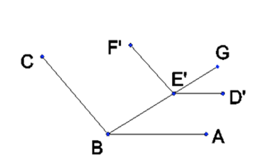
Proof: It suffices to show that the interior angles at each pair of corresponding vertices are equal. Let A, B, and C be consecutive vertices of the bottom polygon and D, E, and F be the corresponding vertices of the top polygon, respectively. By Proposition 2, DE is parallel with AB and EF is parallel with BC. There exists vertices D’, E’, and F’ which are translated vertically from the top polygonal face down to the plane of the bottom polygon. By this we obtain lines D’E’ and E’F’, in the plane of the bottom polygon which are parallel with DE and EF, respectively. By Proposition 1, D’E’ is parallel with AB and E’F’ is parallel with BC. Draw a line through B and E’ to some point beyond E’, say, G (see Figure 1).

Figure 1. AB || D’E’ and BC || E’F’.

Then we have corresponding angles ABE' = D'E'G and CBE' = F'E'G. Thus, ABC = D'E'F'. We take for granted that the translation of DEF to D’E’F’ did not alter the angle between the lines and so we have our result.■

Corollary 3. The cross-section taken parallel with the end faces is everywhere similar to the ends.

Proof: By observing that the parallel cross-section intersects the trapezoidal walls of the prism so as to produce lines which are parallel to the base and top (Corollary 2), the argument applied for Proposition 3 applies here as well.■

Proposition 4.  The lines extended from the side edges intersect at a common point (the apex).

Proof:  Consider three consecutive vertices on the base A, B, and C, and corresponding vertices D, E, and F on an arbitrary parallel cutting plane parallel with ABC. By corollary 3,

Since AD and BE are coplanar, they intersect at some point P. Similarly, BE and CF intersect at some point Q. Assume that P ≠ Q. Take a section parallel to the base through P and label the vertices of the section which correspond to A, B, and C as D, E, and F and observe that the above proportion equation still follows from corollary 3. Also, D = E = P and so line segment DE = 0. However, since P ≠ Q, line segment EF ≠ 0, which contradicts the proportion above. Therefore, our assumption that P ≠ Q is wrong and we have P = Q. By the principle of mathematical induction, the proposition follows.  [Finding P is (i) 2 in S and establishing P = Q is (ii) the inductive step. 1 in S is either automatic or ill-defined I suppose, but irrelevant anyway.]■

The shape we have considered in this post is a frustum of a (possibly slanted) pyramid by proposition 4.

We conclude by noting that the argument for determining the volume of the frustum of a pyramid does not impose a condition that requires the top face to be centered over the bottom face. A slant does not alter the argument and therefore the result is the same. Note, of course, that the height must be measured perpendicularly to the end faces. It should be noted that we have not dealt in this post with the relationship between the cross-sectional area and the height, which relationship is needed in order to establish the volume formula.

Such proof involves 1) similar triangles, using the height of the apex as a reference, and 2) the relationship between linear dimensions and the area(s) they pertain to. Assurance of the existence of a proper apex is the critical component addressed in this post.

Thanks to one of my readers for the question at the end of a previous post that led to this post.

Introspecting the Lisp Representation of a Maxima Variable

I recently wanted to know how Maxima (a computer algebra system) implemented something.  I searched and searched and couldn't solve my problem.  Specifically, I wanted to access a Maxima structure from within Lisp code.  However, I didn't know how the structure was implemented in Lisp and therefore didn't know how to access it.

All you need is a single line of inline Lisp:

:lisp (print $structures)

structures is a global variable which stores the structures that have been defined in the session by using defstruct().  I wasted a few hours looking for this information to come up with 25 characters that would answer my question.  Applying the same general idea to an instance of PanelStruct() tells me how it is implemented.  By the way, the answer to my questions looks like this:

((MLIST) ((|$PanelStruct|) $SIZE $TOP $CENTER $BOTTOM $ZENITH $AZIMUTH |$rdv|) ((|$RayStruct|) $START $DIRECTION) ((|$PlaneStruct|) $NORMAL $CONSTANT) ((|$PanelStruct|) $SIZE $TOP $CENTER $BOTTOM $ZENITH $AZIMUTH |$rdv|) ((|$RayStruct|) $START $DIRECTION) ((|$PlaneStruct|) $NORMAL $CONSTANT)) ((MLIST) (($PanelStruct) $SIZE $TOP $CENTER $BOTTOM $ZENITH $AZIMUTH $rdv) (($RayStruct) $START $DIRECTION) (($PlaneStruct) $NORMAL $CONSTANT) (($PanelStruct) $SIZE $TOP $CENTER $BOTTOM $ZENITH $AZIMUTH $rdv) (($RayStruct) $START $DIRECTION) (($PlaneStruct) $NORMAL $CONSTANT))

The near repeat is caused by the print function returning what it has printed and Maxima outputting it.  The $ indicates a references to a Maxima variable and the | | symbols indicate a case sensitive reference.  Oddly, the case is reversed for RDV (which is documented) but not for PanelStruct which surprises me.  (These structures are not built-in but were user-defined in my Maxima session.)

I will still need to figure out how I'm going to use the information, but I have a working concept.

Lighting Distribution

I've written a simple Maxima program which uses linear interpolation and lamp luminous intensity data to determine the illuminance on a flat surface (read floor or work surface) caused by several lamps in different locations.  It displays a color contour do show you how the light is distributed.  I could probably tweak some things to get a nicer selection of colors for the color contour but as far as a result which is easy to interpret, this works fine.  Behold:

Never mind the clutter in the bottom left hand corner.  This is just the z-axis numbers written on top of one another because we are looking straight down on the graph.  Small price to pay for the cool result and you can edit the picture afterward if you need something for presentation purposes.  An additional problem I observe is the aspect ratio.  It should look square because my chosen room is square (8' × 8').  Dauntless, I press on.

To implement this program with your own example you need:

• Maxima:  a free computer algebra system.
• Light data
• A room and light configuration.

Light Selection
You need to select a light and find the manufacturer data.  I am using the Cooper RPN3MR-E3MRC.  This is a combination of the light fixture and the lamp in the fixture.  The data you need will indicate how the candle power changes with vertical angle.  The assumed situation is that the light is pointing down.  The vertical angle is measured between the vertical line passing through the center of the light fixture and the line drawn through the center of the fixture to a location on the floor (or incident surface).  This vertical angle affects the "amount of light" (measured in candelas) that is going in that direction.  To input the data for your luminaire-lamp combination you enter it on the line that says "lampData:".  The data is in the form of a list of lists where the nested lists (two items each) represent points.  The pattern for each point in the master list is [angle in degrees, candle power in candelas].  If your data doesn't go all the way to 90 degrees, then put a final point [90, 0] to indicate there will be no light going in that direction.

Considerations in the Calculation
The vertical angle not only affects the "amount of light" in that direction but the angle of incidence with the floor.  We are assuming the light is "facing" the floor.  (The floor is horizontal.  The light is shining straight down onto it, although, of course it "spreads out" as it goes down.)  Remembering that the "angle of incidence" is measured relative to the normal line (perpendicular to the floor), you can see that the angle of incidence is an alternating angle with the vertical angle and therefore equal to it.  An angle of incidence affects how the light "spreads out" across a surface because the same amount of light gets spread out more if the surface is at an angle (not "facing head on") to the beam of light.  Also, not every point of the floor is the same distance away from each light.  As light travels it spreads out in two directions.  If you spread the same amount of anything (sound, light, peanut butter) over a larger area, there isn't as much of it in a given area.  The basic formula is:

\[fc = \frac{cp}{d^2}\cos{\theta}\],

where
      fc = foot-candles (a measure of illuminance: cd/ft²)
      cp = candle power (candelas: cd, same unit in metric and imperial, relates to the Watt)
      d = distance (in feet)  
      θ = angle of incidence (measured from the normal).

The formula is the same if you use metric, but the units change.  Instead of entering feet and getting foot-candles, you enter meters and get lux.  You use the same lamp data which is in candelas.  Candelas are the same in metric and imperial.  To put it very simply:

lux = cd/m²
fc = cd/ft²

Using the Program
If you want metric, enter all distances in m (you will get lux).  If you want imperial, enter all distances in ft (you will get foot-candles).

1. As always, choose a coordinate system and stick to it.  Pick a corner of your room to be (0,0) and one of the sides to be the positive x-axis.
2. Enter the length and width of your room.  I have called these x_length and y_length to avoid misunderstandings based on the usual understanding of width < length.  Just pick a dimension to be the x direction length and one for the y direction length.  Doesn't matter which is set to which.  Just be consistent with step 1.  Sorry, only rectangles.  You're welcome to program something more interesting if you get bored some day.  Or, maybe your room can pretend to be a rectangle?
3. Enter the locations (positions) of your luminaires.  These are in terms of [x, y, z].  I have entered the height of the luminaires for the the z value (12.5 feet).  You could instead enter their height above a work surface (the results would only be correct for the work surface).  Alternatively, you can change the Illum(x,y) function definition to use a z-value of the height of the work surface instead of 0 (same caveat as previous suggestion).

load(interpol); x_length: 8; y_length: 8; luminairePositions: [[2,2,12.5],[6,2,12.5],[2,6,12.5],[6,6,12.5]]; lampData: [[0,2513],[5,1922],[15,1052],[25,406],[35,43],[45,5],[55,0],[90,0]]; f(x) := ''(linearinterpol(lampData,varname='x)); P2P_Illum(x,y,z,lampPos,lampCandelaFunc) := block( h: float(sqrt((lampPos[1]-x)^2+(lampPos[2]-y)^2)), d: float(sqrt(h^2 + (lampPos[3]-z)^2)), theta: float(180/%pi * asin(h/d)), cd: lampCandelaFunc(theta), return(float(cd/d^2*cos(%pi/180*theta))) ); Illum(x,y):=sum(P2P_Illum(x,y,0,luminairePositions[i],f),i,1,length(luminairePositions)); plot3d(Illum, [x, 0, x_length], [y, 0, y_length],[mesh_lines_color, false], [elevation, 0], [azimuth, 0], [colorbox, true], [grid,80,80]);

Note:  P2P_Illum() means Point-to-Point Illuminance.  Illum() is the sum of the illuminance contributions of each luminaire to a given point.

Possible Improvements to the Program

1. Change the color selections for the plot.  Perhaps yellow for higher values.  Might be a fiddly thing to get right.
2. Include a more explicit boundary (wall) definition mechanism.  A list of vertices would satisfy the wall definition needs.  But then some programming would need to be done to determine which lights have a line of sight to a given x,y point.  There would also be a need to either crop the end result or indicate some neutral value for places in the plot area but not within the boundaries of the room.
3. Allow the incident surface shape to be specified.  
• This might be as simple as allowing inputs of areas at different heights.  This would be the simplest and most widely useful approach.  It would be helpful to indicate the locations of the different surfaces on the plot as well.  It might be necessary to directly use the draw package to do this. [First, load(draw).  Then learn how to use draw.  I haven't looked much into it yet.]
• More complex surface entry would require more complex angle of incidence calculations.  The angle of incidence would not necessarily be equal to the vertical angle.  If the incident surface (or part thereof) was represented as an analytic function of two variables, you could use the partial derivatives to determine the tangent plane and thus the direction of the normal.  Given the direction of the normal and the direction toward a given luminaire, you take the dot product of these (normalized/unit) vectors to get the cosine of the angle of incidence (which is what you need; see formula above).

Degree of Saturation versus Relative Humidity

These two quantities are similar and as I worked through ASHRAE Handbook Fundamentals (2009) IP, chapter 1, I was initially baffled as to what the difference was.  First, the definitions based on ASHRAE Fundamentals:

Relative humidity:  The mole fraction of water vapour in a sample divided by the mole fraction of water vapour in saturated air at the same temperature and pressure.

Degree of saturation:  The humidity ratio of water vapour in a sample divided by the humidity ratio of water vapour in saturated air at the same temperature and pressure.

Humidity ratio:  The humidity ratio is the mass of water vapour divided by the mass of dry air in a sample. This value can also be expressed in terms of molar fractions.

Discussion of Differences

In relative humidity, imagine taking two samples, one of the air which you want to know the relative humidity of and one of saturated air at the same temperature and pressure. For example, we might take samples of 1 mole each. In the non-saturated air, we will have less water vapour than in the saturated air. On the other hand, we will have more dry air in the non-saturated sample than in the saturated sample. The same general relationship will be true of mass, but the masses and the mole fractions will relate differently due to differing molecular masses. Here's the bottom line: we compare the samples based on moles (which amounts to the number of molecules) not on a given mass or volume. When you're dealing with gases, moles is the way to go.  In other words, our non-saturated and saturated samples relate by the equation:

where the items on the left hand side are the mole fractions of water vapour and dry air in the non-saturated sample and the items on the right hand side are for saturated air.

Understanding that we need to compare these quantities with a fixed number of total moles as in the previous equation is what makes ASHRAE's equation (14) work out.  From the last given equation we have

Therefore,

which verifies equation (14) as given in ASHRAE Fundamentals (2009).

It is worth noting that we only had to worry about this molar equality in developing this equation. When it comes to computing the degree of saturation from the relative humidity and vice versa, we don't have to think about that. The formula will do that for us. Also, we can still compute the degree of saturation directly from values off of a psychrometric chart (for example) by reading across to the right to get \(W\)and finding \(W_S\) by finding where the dry bulb temperature intersects the saturation curve and reading across to the right.  The definition of degree of saturation doesn't require us to account for the number of moles, only the relative humidity (and yes, if you're using charts you can read it off there as well).  If you are familiar with reading psychrometric charts, you will know that reading W values is generally much easier than reading RH values.

So if you're getting different values for these quantities in your work, it's not (necessarily) a mistake or a misreading of the chart—they really are different.