iMaxima and Slime in EMACS

First of all, I am a Windows user. Lots of (probably) very helpful documentation for how to do this is not directly applicable to my setup, because I am not a Linux user. Bummer. That being said, it worked out in the end.

If you just want to hurry up and try Common Lisp in a REPL, then try Lispbox.

I recently set out to do two things:

1. Get EMACS to run Slime (with any Common Lisp implementation)
2. Get EMACS to run iMaxima

Slime

Watch Installing Common Lisp, Emacs, Slime & Quicklisp: It's a demo of installing EMACS with SBCL, Quicklisp, and Slime.

• The primary hangup I was having until I saw this video is that I was trying to find a way to get EMACS to do something that I was supposed to do from within a running instance of a selected Common Lisp implementation. In other words, if you want to use CCL in EMACS using Slime, you should run CCL in a cmd window and use that REPL. Like many solutions, it's totally obvious when it is shown to you, which is why you may have trouble finding explicit statements about this.
• If you want to see a few of the basic environment variable modifications in slow motion (as it were), see here.

To start slime, I launch EMACS and then type ALT-X slime ENTER.

iMaxima

Visit the main site for iMaxima to see what it's about. It also has a section for installation instructions. Most of what you need to know is on that website. Below are details from my own setup and additional research that helped me get the system up and running on my computer.

After you have EMACS setup and have decided your HOME folder (see here), run EMACS to let it create a ".emacs.d" folder. Then create or edit the file init.el (el means EMACS Lisp, I believe). Here is my entire init.el (largely excepting comments), which includes commands for a REPL with SBCL and iMaxima (separately):

(load (expand-file-name "~/quicklisp/slime-helper.el")) ;; Replace "sbcl" with the path to your implementation (setq inferior-lisp-program "sbcl") (add-to-list 'load-path "C:/Program Files (x86)/Maxima-5.31.2/share/maxima/5.31.2/emacs") (load "setup-imaxima-imath.el") (autoload 'maxima-mode "maxima" "Maxima mode" t) (autoload 'imaxima "imaxima" "Frontend for maxima with Image support" t) (autoload 'maxima "maxima" "Maxima interaction" t) (autoload 'imath-mode "imath" "Imath mode for math formula input" t) (setq imaxima-use-maxima-mode-flag t) (add-to-list 'auto-mode-alist '("\\.ma[cx]" . maxima-mode))

Size of TeX output can be modified using (setq imaxima-fnt-size "xxxx"), where xxxx is one of small, normalsize, large, Large, LARGE, huge, or Huge. Also, by viewing the imaxima.el file, you can see a number of other options that are available to you.

To understand what's happening a bit better, it helps to know a few variables.

1. Go to your scratch buffer in EMACS.
2. Type inferior-lisp-program CTRL-j.
3. You will get the output "sbcl" if you used my init.el file.

I suggest the scratch buffer because it is important in debugging when you don't have a working setup of anything else. The scratch buffer is available. It runs ELISP, EMACS' own Lisp dialect.

Here are a few other variables you might benefit from looking at:

• load-path
• exec-path
• image-library-alist

I've bolded image-library-alist because it is really helpful to know what file you need to display png files. I snagged the files jpeg62.dll, libpng14-14.dll, and zlib1.dll from a couple of sources and placed them in "C:\Program Files (x86)\emacs-24.3\bin" which is where my "runemacs.exe" is. 

• Notably, I got libpng14-14.dll and zlib1.dll from "C:\Program Files (x86)\Inkscape". (You really should try Inkscape, the free SVG editor, anyways.)
• If your image-library-alist has other files in it, you either need to augment your image-library-alist (probably in your init.el file) or find one of the files already in image-library-alist and place it in the load path. You only need to do this for png files (as far as I know) in order to use imaxima.

A command you should try running (still in the scratch buffer) is

    (image-type-available-p 'png)

which will return T or NIL depending on whether the file type is available or not, respectively. If you get NIL, it means you don't have one of the files in image-library-alist in your load-path (or perhaps a dependee file is missing?).

Breqn

I had a lot of trouble with the display of the LaTeX even after I had a running imaxima session in EMACS. (Results of evaluations are usually displayed with LaTeX.) The problem stemmed from a missing package: breqn. I installed the mh package from within the MiKTeX Package Manger and it appeared to install fine, but my LaTeX was still not working properly within an imaxima session. The issue appears to have been related to dynamic loading of packages.

Here's what finally shook the problem loose: within TeXnicCenter I started a new project and included the line

    \usepackage{breqn}

along with the other \usepackage declarations that were part of that project. When I built the project I was prompted for the installation of the package and the installation appeared to go smoothly. Then I tried imaxima again and the LaTeX output worked.

To start an imaxima session, launch EMACS and then type ALT-x imaxima ENTER.

Piece of cake! :)

Additional Info (probably not necessary)

I'm still getting a warning message when I load imaxima, although it has yet to prove to be a problem. The warning is:
   (lambda (x) ...) quoted with ' rather than with #'

I also made another change, and I don't know if it was necessary or not (hopefully not), but while wrestling with something quite different I changed line 14 of maxima-build.lisp (that's "C:\Program Files (x86)\Maxima-5.31.2\share\maxima\5.31.2\src\maxima-build.lisp" on my system). I changed that line to:

(load "C:/Program Files (x86)/Maxima-5.31.2/share/maxima/5.31.2/share/lisp-utils/defsystem.lisp")

This is just an explicit file reference rather than a relative path. (In case you're wondering, I was trying, unsuccessfully, to compile maxima myself. Perhaps another time.)

Skew Cut Profiles

I recently was surprised (anew) at what happens when you cut a prism which has a uniform cross-section with a plane which is not orthogonal to the length of the prism. Especially if the plane must be described in terms of two angles. A cross-section through a square prism is (by definition) a square. If you make your cut at an angle, you will get a rectangle if you have a simple angle cut. But if you make your cut not only a miter, but also a bevel you end up with a parallelogram.

The simplest way to visualize this is to imagine a plane that intercepts the prism at a single edge first and has its steepest slope in the direction of the opposite edge:

The resulting section when viewed in the intersecting plane would be something like this:

where the blue square is the cross-section, the red parallelogram is the intersection of the above described plane through the square prism when viewed in that plane. (A few thought experiments of your own will probably serve you better than any further illustration of this phenomenon I could drum up at the moment.)

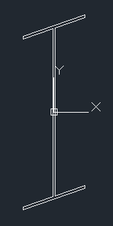
It is interesting to see the result in an I-beam shape if you use a 45° miter and 45° bevel:



As a matter of where this observation fits into mathematics generally, this is a projective or affine transformation. Such transformations preserve straight lines but they do not, in general, preserve right angles.

Aside: Convex Hulls

The fact that they preserve straight lines is a boon to the would-be-writer of a convex hull algorithm in an arbitrary plane since you can project the 3D coordinates onto a simple 2D plane and use the 2D algorithm (being careful to preserve or restore the other coordinate at the end). If you do so, you should probably choose which set of 2 coordinates to use for the algorithm, based on the direction of the plane. For example, if the normal of the plane has a larger z-coordinate than x- or y-coordinates, then the (x,y) pairs are best to use for the information to run the 2D convex hull algorithm on. There are two reasons to be picky about this:

1. If the points fed to the routine are in thy yz-plane, you will get incorrect results (if you assumed the (x,y) coordinates should always be used).
2. It may reduce the effect of rounding errors in the calculations (in terms of deciding whether points "near the line" of the hull are inside or part of the hull).

(I have lost the original code I used for this post, so I omit references to it now.)

See the Maxima project for download information for Maxima.

Round 'em up!

Over the past several months I have been dabbling in Common Lisp (LISt Processing language).  Lisp, I think, is the ugly duckling of the programming languages. The facetious "Lost In Stupid Parentheses" seems more apt as an acronym.

My first encounter with this ungainly language (Lisp) was in AutoLisp (and Visual Lisp). I was on a hiatus from programming regularly and discovered this immediately discouraging language that was the "easiest" way to interact with AutoCAD programmatically. (I don't consider AutoCAD scripts to be programming, though I would still include them under the more general category automation.) I did not make much headway at that time and it frankly amazes me that any non-programmer will step up to the challenge and learn it.

But then there was Maxima. I was happy with Maxima as a free computer algebra system. But in the documentation I found the spectre of Lisp. Specifically, Common Lisp. The computations in Maxima are all in Lisp (though there is probably some non-Lisp they use to glue together a Windows interface for Maxima). Maxima itself supports a fairly robust set of programming constructs as far as doing calculations are concerned.

• Input/output from files
• Controlled loops
• if-then-else
• functions
• plotting (via gnuplot—included in standard installs)
• formatted output
• nice math notation display
• export to latex or image

Maxima is built on top of Lisp and you really have all the abilities of Lisp in Maxima (if you know how to get at them). But, being as I am, always in search of a better way of doing something, I am also concerned with whether a technology built on top of another is "hiding" some of the features of the underlying technology. Perhaps hiding isn't exactly the right way to put it, but learning Lisp is a paradigm shift from most other (Algol-like) programming languages I was familiar with, while on the other hand, learning Maxima didn't take me through that paradigm shift.

The two most interesting features of Lisp to me are the emphasis on function references and macros. But they both help you to do the same thing: reduce the repetition in your code. Mind you, they serve this end in very different ways.

When I wanted to implement Jarvis's march [1, p. 955] to encircle a list of points in a "convex hull" it was particularly the function referencing that made the implementation of the code fairly simple.

Fig 1. The red lines join together the red + signs which indicate the convex hull for these points.

The general idea of Jarvis's march is you find an outside point to start from and then keep picking the next point so that you never have to switch directions as you walk around. I started at the left most point. In the event of a tie, I choose the lower of these. (That would place us at about (0.1, 15.0).) I decided to walk around the points in a counter-clockwise direction. To decide which point comes next, I need to find the point which requires the right-most turn. So I begin by choosing the first of the remaining points (in whatever order I received them). I go through the remaining points and test whether I would need to make a right turn or left turn to point toward them (from my vantage point on the starting point of the hull chosen at my first step). If it is a right turn, then I have a new winner which replaces the first and I continue moving forward to the points not yet checked. The algorithm is really a repeated application of a maximum function where maximum is defined according to a different function than normal. What I need are predicate functions which define the rules for choosing a winner (a "maximum") and a routine to separate the winner from the remaining points that can accept a predicate function as a parameter.  Here's the code for, remove-winner:

(defun remove-winner (test li) (let ((mx (car li)) (temp nil) (therest nil)) (setf therest (loop for i in (cdr li) collect (if (funcall test i mx) (progn (setf temp mx mx i) temp) i))) (list mx therest)))
The idea of remove-winner is to use the test function (supplied by the caller) to determine whether the next item is "better" than the current winner. If you passed in the function < (using the syntax #'<) you would get the smallest value in the list (provided it was a list of numbers). Notice the thought process in this function is not just to find the max and return it, but rather to produce a list which includes the "winner" and the rest of the values (that didn't win) separately. We don't just need to know the winner, we need to separate the winner from the rest.

When we get to the convex-hull routine, we can use the same routine (remove-winner) using two different tests: one to find the initial element and another to find the successive elements.

(defun convex-hull (points) (cond ((< (length points) 3) (list nil points)) ((= (length points) 3) (list points nil)) (t (do* ((init (remove-winner (lambda (a b) (if (= (aref a 0) (aref b 0)) (< (aref a 1) (aref b 1)) ;; pick the lower (< (aref a 0) (aref b 0)))) points)) ;; pick the lefter (start (car init)) (rest (cadr init)) (next nil) (hull (list start)) (result nil)) ((or (eq start next) (not rest)) (list hull rest)) (setf result (remove-winner (lambda (a b) (right-turn-from (vect- a (car hull)) (vect- b (car hull)))) rest)) (setf next (car result)) (if (right-turn-from (vect- start (car hull)) (vect- next (car hull))) (setf next start) ;; set terminating condition (progn ;; else (setf hull (cons next hull) rest (cadr result))))))))

The first occasion we use remove-winner, the function is of the same sort we would use to perform a two key sort. In the main body of the routine, we have a more interesting function which accepts two points, calculates their direction vectors (using the current head node of the hull as the origin) and decides whether the second is a right turn away from the first, in which case it declares the second to be the (current) winner.

Can you do this [abstract the predicate] in other languages? Yes. In many other languages you could implement the routine substantially like this. But the key is this: would you ever think to do it this way if you were using VB.NET or C# or C++? Maybe. But not because of your experience with those languages, but because of your experiences with Lisp or F# or other languages which feature a functional style of programming.

Fig. 1 was produced from running a small bit of Maxima code which loads some routines from a separate package written in Lisp (including the above routines).  You can download both files to try them out:

• points.lisp
• circlethempoints.wxm

You will need to have Maxima installed to try this example out.

Sources:

1. Cormen, T.H., Leiserson, C.E., Rivest, R.L., & Stein, C., Introduction to Algorithms, Second Ed., McGraw-Hill Book Company / The MIT Press, 2001.

Sum of Powers

In the sum of powers problem, we are looking for the sum of the p^th power of the first n integers. In this post, we consider the problem of determining a polynomial expression in n for a given power. The best known case is for p = 1, namely,

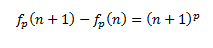
More generally, we should like a formula for a polynomial f_p such that

We will begin by defining a function and proceed to prove that it satisfies the above equality. We define:

Proposition 1. For all real numbers \(n\) and natural numbers \(p\),

Proof:  First we observe that (n + 1) – n = 1 = (n + 1)⁰, so that we have our induction base set. Suppose that for any real number n > 0 and a given natural number p we have,

Now, given any real number n > 0,

which completes the argument.■

Proposition 2. For all natural numbers \(n\) and \(p\)

$$f_p(n) = \sum_{i=1}^n{i^p}$$

Proof: First we see from the definition both that \(f_0(1) = 1\) and, for any \(p > 1\)

$$f_{p}(1) = p \Big(\int_0^1 f_{p-1}(x) \mathrm{d}x - 1 \int_0^1 f_{p-1}(x) \mathrm{d}x\Big) + 1 = 1,$$

which establishes \(1 \in S\). Suppose that \(n \in S\). Then

$$f_p(n) = \sum_{i=1}^n{i^p},$$

and from proposition 1

$$f_p(n+1) - f_p(n) = (n + 1)^p$$

which rearranges to

$$f_p(n+1) = f_p(n) + (n+1)^p$$

$$= \sum_{i=1}^n{i^p} + (n+1)^p  = \sum_{i=1}^{n+1}{i^p}$$

■

The formula we have given for f_p allows us to calculate the first p sum of powers polynomials in time O(p²) which is a big improvement when compared to solving a system of linear equations to find the largest of them, which would require time O(p³) (to find all of them using a system of linear equations requires O(p⁴)).

The following Maxima program and its output, gives a demonstration of how to implement the above formula:
f[0]: n$ for p: 1 thru 100 do ( f[p]: integrate(expand(p*f[p-1]),n), C: 1 - ev(subst([n=1],f[p])), f[p]: f[p] + n*C )$ [f[0],f[1],f[2],f[3],f[4],f[5]];

[n,n^2/2+n/2,n^3/3+n^2/2+n/6,n^4/4+n^3/2+n^2/4,n^5/5+n^4/2+n^3/3-n/30,n^6/6+n^5/2+(5*n^4)/12-n^2/12]

The Un-Pyramid

In previous posts I've discussed truncated pyramids and irregular triangular prisms, but I hadn't at that time thought to consider a "really irregular triangular prism" before.  I was searching on the general notions of these topics on the internet to see what people were thinking about with respect to them and found someone had something different in mind:  A 5 sided solid with a non-constant triangular cross-section and no faces (guaranteed) parallel with each other.

The first thing to note about this shape is the characterization of the faces.  The two "ends" are triangular faces. There are three quadrilateral faces which form the boundaries of the non-constant triangular cross-section. The three edges shared by the quadrilateral faces are not parallel with each other and the quadrilaterals could be completely irregular. Here is a quick video of a Sketchup model of just such a shape:


The Un-Pyramid from Darren Irvine on Vimeo.

Since the consecutive pairs of "side" edges are part of a quadrilateral (they are proper "faces"—no twists), they are certainly coplanar. In a previous post, I demonstrated that two parallel faces with edges joining corresponding vertices with consecutive edges being coplanar, the parallel faces are necessarily similar. I also demonstrated (Proposition 4) that the projected side edges intersect at a common point, which we may call the apex.

The un-pyramid does not have the two parallel faces that formed the starting point in that post. However, it does have the consecutive coplanar edges. And although we have not been given a "top" face parallel with the bottom, we can certainly make one. We establish a cutting plane through the closest vertex (or vertices—there could be two at the same level) of the "top" face which is parallel with the larger "bottom" face. (We can turn the un-pyramid around to make the names fit if it comes to us upside down or sideways.) Now we can be sure that the side edges can be projected to a common apex as per 3D Analogue to the Trapezoid (part 3).

Fig. 1.  A really irregular triangular pyramid? Hmm...

Calculating the volume of this shape requires a bit of calculation just to figure out how to break it up into pieces. If you want to program a solution to this problem, you are probably going to take in A₁, B₁, C₁, A₂, B₂, and C₂ as the parameters. To verify you have valid data establish that:

• A₁A₂ is coplanar with B₁B₂
• B₁B₂ is coplanar with C₁C₂
• C₁C₂ is coplanar with A₁A₂
• Also, make sure these same edges don't intersect each other (meaning the lines projected through them should intersect outside of the boundaries of the line segments).

You also need to determine whether the apex is closer to A₁B₁C₁ or A₂B₂C₂. Then reorder or relabel the end faces as necessary. The face further away is the base (say ₁). Now determine which of the top vertices is closest to the base and establish a cutting plane through it, parallel to the base.

(Hint: It will be convenient to reorder or relabel your points so that A₂ is the closest point, B₂ next, and C₂ furthest; this avoids polluting your code with cases. Don't forget to reorder the points in the base. You may have a job making the relabeling of previous calculation results work properly. Making clear code that does minimal recalculations is probably the most challenging aspect of this problem if treated as a programming challenge.)

Now we can calculate the volume as a sum of two volumes:

1. Frustum of a (slanted) pyramid with base A₁B₁C₁ and top A₂BC.
• For the overall formula, see 3D Analogue to the Trapezoid (part 2)
• To find the areas of the top and bottom, use the cross-product method (see Area of Triangle Given Coordinates)
• To find the height, find the component of vector (A₂ – A₁) perpendicular to the base (also used in Volume of a Tetrahedron)
2. Slanted pyramid with base BB₂C₂C and apex A₂
• Find the area of the base
• watch out for B = B₂ and C = C₂ which changes the shape of the base
• If both are true, then you've dodged the bullet—there's no volume to worry about.
• If B = B₂, then either it is at the same level as C₂ or the same level as A₂. But in either case, you have a triangular base.
• Very possibly neither of these will be true. Break the quadrilateral up into two triangles using the diagonal of your choice.
• Find the height of the pyramid using the component method as for finding the height of the first volume.

But, what should we call it?

1. triangular un-pyramid
2. really irregular triangular prism
3. skew-cut slanted triangular pyramid
• alternatively, skew-cut slanted pyramid with triangular base

I guess I like 1) for the advertizing, 2) for the baffling rhetorical effect, and 3) for half a hope of conveying what the shape really is.

Find the Intersection of a Plane with a Line

We can represent a plane with four numbers, the coefficients of the general equation of a plane, as ax + by + cz + d = 0.  For convenience, we can represent this also as

where n = (a, b, c) and r = (x, y, z) is a point on the plane.

We take a line through two points, A and B, in vector form as

        L(t) = A + (B–A)t

We want to find the intersection of the line with the plane.  That is, we need f, such that

Then,

And so

The desired point is L(f), since it on the plane and on the line.

Notice that the calculation of f requires only the evaluation of the general equation of the plane using A and B as the points. The results will not be zero unless A and B are on the plane, in which case we would already have the result. If the line is parallel with the plane, then the denominator will be zero giving an indeterminate result. This fits with the geometric interpretation of the plane evaluation. The point of the last step in our derivation is that it simplifies the coding of the problem somewhat by reducing it to two plane evaluations. (If you observe carefully, you will see it makes the difference not of two additions but only of one.)

Evaluating the equation of a plane using a point not on the plane gives a result which is proportional to the distance between the planes. If the normal vector (n = (a, b, c)), has a magnitude of 1, then it yields the distance. However, in the formula we have derived, we have not depended on the equation of the plane being normalized. The constant of proportionality in the numerator cancels with itself in the denominator (I mean "behind the scenes" or if you derived it using a different approach) to produce the simple result for f above.

The idea for this solution came from initially viewing it as a linear interpolation problem, which, of course, it is. Similar triangles also are an acceptable approach the problem, though it may be more difficult to deal with the signs. The above derivation deals with sign transparently.

Convective Heat Transfer: Buildings in the Cold

Engineering Toolbox has an equation (here) for calculating a convective heat transfer coefficient:
   

where v is the wind speed in m/s and h_c is in W/(m² K).  When I first found this equation I thought that I had a way to calculate the h_actual/h_NW ratio more accurately than in my earlier post about "wind chill" on buildings.  As I reviewed my previous post however, I realize that this is awkward to compare.  The ratio that I would obtain using the above equation is h_actual/h_NW = 2.833 (this is comparing convective heat transfer with 15 mph wind versus no wind).  To see that something isn't quite copacetic, observe that if we use the equation used there, namely,

       T_WC = T_S – (h_actual / h_NW)(T_S – T_actual)),

with 2.833 for the ratio and 88 °F as the skin temperature, we obtain

    T_WC = 88 – (2.833)(88 – (–31)) = –249 °F,

the implausibility of which suggestion I am satisfied. Radiative heat loss may be complicating the situation. But whatever the reason, the wind chill equation makes no promises to us about its applicability to anything other than humans.

The current day wind chill index is a bit of a backward way of looking at things. Notice that it is called an index. It is not a physical quantity. It is a measure of a phenomenon. The wind doesn't make the temperature outside colder.  It does make bodies which are warmer than the air loose heat faster. But be cautious with relative terms. Something does not really loose heat "faster".  Rather, it may lose heat "faster than something else". It is more helpful (to the understanding) to say that the absence of wind results in a building loosing heat less quickly than a wind swept building.

I say this because of the way one sets up the steady state heat equations. We set the temperature of the outside of the outer air film to be equal to the ambient outdoor temperature. And we assume a small air film with R value something like 0.15 so that the outside surface of the building is not much different in temperature than the ambient air temperature. However, this neglects the affects of sunlight. In the absence of wind, sunlight has the most beneficial effect to the exterior of a building (in winter). By heating up the exterior surface of the building, the thermal gradient across the envelope is less—there is less temperature difference from inside to outside—and therefore the rate of heat loss through the envelope is reduced. The benefit of sunlight is kept in check by the convection on the outside of the building. As the exterior of the building gets warmer, the temperature difference between it and the air increases, which increases the rate of heat loss from the surface of the building.  If there is significant wind, it will mean a larger convective heat transfer coefficient (relative to no wind) and therefore raise the rate at which exterior surface loses heat, which in time reduces the temperature difference between the air and the exterior surface.

Hence, in modeling a steady state temperature loss, the coldest the outside temperature of the envelope should be modeled at is the ambient outside temperature; this is the worst case scenario. To see that this is true, notice that at this point there is no temperature difference between the ambient and the exterior surface. Considering the convective heat transfer equation, this means there is no heat transfer. Thus,

       q = h_c·A·(T_S - T_air) = h_c·A·0 = 0,

by which observation, with some thought, you might realize that this means the outside surface is necessarily warmer than the ambient air temperature, by at least some amount. Otherwise your building would stop losing heat, which would be very efficient indeed if it was possible!

If you want to model the benefits of reduced wind conditions and sunlight, you might model the exterior temperature as being warmer than ambient.  In short, wind lessens the benefits of sunlight to the thermal performance of a building envelope, but it does not make the exterior colder than ambient.

What I am saying is that the reason why heating requirements may be higher in windier places is because the less windy places are receiving (and retaining) a greater amount of benefit from sunlight and therefore have lesser heating requirements.

If Not "Wind Chill", Then What?

If the wind chill index is not totally real (though it is fine for its intended purpose), what should we be considering? The physical quantity that really matters is called heat flux. Heat is the transfer of thermal energy (1, p. 53). Of course, when a transfer is happening, it is happening at some rate.  So you can speak of loosing or gaining heat at a rate specified in Watts, kilowatts, Btu/h, etc. Heat flux is the rate of thermal energy gain/loss per unit time and area.  Possible units of measure include W/m² and Btu/(h ft²).

Solar radiation is often expressed in these units.  Note however, that to model the effect of the sunlight effectively requires you to determine the fractional portion of the incident radiation which is actually converted into thermal energy. You also need to scale the result by the cosine of the incidence angle (measured perpendicular to the surface normal) since a non-direct (non-normal) angle "spreads out" a given amount of radiation over a broader area.

One of the merits of working with heat flux, is that you can compare a tendency to heat loss between objects of varying surface area. A really large building might be losing heat faster than a small building even though it is better insulated. If you wanted to compare their tendency to loose heat on a kind of level playing field, you would divide the rate of heat loss by surface area.  Your result would be heat flux—actually, average heat flux.

If you want to calculate heat flux (φ), divide area out of the convective heat transfer equation:
   

(For the convective heat transfer equation, see ASHRAE Fundamentals chapter 4 or [1].)

But we have now touched on an important issue in energy efficiency: bigger isn't always better. If you can reduce your volume, you reduce the amount of stuff to heat.  (This is most pertinent in spaces with redundant air space, where the hot air rises to the top and is useful only for increasing the rate of heat loss through your roof—and when I say useful, I mean not useful.)  If you reduce your surface area, you reduce the area through which you lose heat. If you don't need big, go small. After you decide the space you really need, configure the space to reduce exterior surface area, subject of course to meeting the functional requirements of the space.

An interesting case of balancing surface area with other considerations is in solar energy greenhouses (SEGs).  A long building a few meters wide with a broad glazed wall facing south (up here in Canada) allows the building to maximize the amount of sunlight captured and stored in the north thermal mass wall. A square footprint would reduce the surface area for a given volume, but it would result in redundant air space. (Plants at the south wall would be too far from the north wall to benefit from it and the roof would need to be higher to allow the sunlight to reach the north wall.)  For more information on these greenhouses, see [2] and [3].

Sources:
1. World of Energy, Chapter 4: Transfer of Thermal Energy, http://www.physics.ohio-state.edu/p670/textbook/Chap_4.pdf
2. Bomford, M., Solar greenhouses, Chinese-style, http://energyfarms.wordpress.com/2010/04/05/solar-greenhouses-chinese-style/, 2010
3. Love, M., The solar solution, http://www.greenhousecanada.com/content/view/1562/38/
4. Wind Energy Institute of Canada, Wind Chill Temperature Index, http://www.weican.ca/links/011101-ec-windchill-index.php
5. Engineering Toolbox, Convective Heat Transfer, http://www.engineeringtoolbox.com/convective-heat-transfer-d_430.html
6. Irvine, D., Convective Heat Transfer on a Building Envelope (Wind Chill?),  http://darrenirvine.blogspot.com/2012/12/convective-heat-transfer-on-building.html, 2012