Using the LispWorks' CAPI, I have implemented a simple program to demonstrate the basic elements in the implementation of a 2D dynamic zoom feature. The program is basically uninteresting except for the dynamic zoom implementation. You can start with the code immediately, or skip to the other side for a few comments and refer back.
Every time the user clicks the left button (:button-1), the mouse location is trapped and turned into a "model" location for a line starting position. If the user presses the right button (:button-3) the common terminal point for all of the lines is changed—the same principle of storing a "model" point is followed. Basically it is a spider with as many legs as you want originating from whatever point you select.
When the program commences, the top-left corner is (0, 0) and view scale is 1:1. The rolling of the scroll wheel of the mouse will change both of these parameters by scaling relative to the current location of the mouse pointer. Since the scroll event does not appear to provide a means to get the current mouse pointer location, I am tracking the mouse :motion "gesture" (basically an "event") and storing the pointer location, in screen coordinates, as is moves.
The change-start (I guess I should have said "add-start"—ah, scope creep) and change-center handler functions do basically the same thing. Using the current mouse position (these two handlers do receive mouse position information), determine the model point corresponding to the screen position of the mouse. The top-left corner is an actual ("model") location. So the model location that corresponds to the given screen coordinates is the top-left corner plus the model distance between the mouse pointer and the top left corner of the screen. Thus, \(M' = (M/s + TL)\), where \(M'\) is the model location. We manipulate the same formula to obtain screen coordinates (\(M\)) from the model coordinates when we display to the screen.
The part that is a little trickier is to adjust the top-left corner when dynamic zoom is applied so that you can maintain the mapping between model and screen coordinates. This is an important part of change-scale's job. Our basic formula is
$$TL_i + A_i = TL_f + A_f,$$ where \(TL_i, TL_f\) are the initial and final top-left corners (i.e., before and after zoom) and \(A_i, A_f\) are the initial and final distances between the model position of the mouse and the top-left corner. In other words, zooming does not change the mouse location in either screen or model coordinates. Hence,
$$TL_f = TL_i + A_i - A_f = TL_i + M {{s_f - s_i}\over{s_f s_i}},$$where \(s_i, s_f\) are the initial and final scale factors.
LispWorks Personal Edition for non-commercial use is available here: http://www.lispworks.com/downloads/.
Monday, April 6, 2015
Saturday, December 6, 2014
What is the Sine of 18°?
To find the exact values of sine (and cosine) of a given angle, you need to use identities. This particular value is interesting in that it takes a fair bit of work to arrive at this value analytically, and yet the value is expressible as a fairly simple radical. The first thing to notice is that 90 = 5(18). You probably know the half angle identity, but not a fifth angle identity. And for good reason—the fifth angle identity has multiple solutions; it's a fifth degree polynomial.
I did this calculation manually the first time through—some years ago. It goes a lot easier with a computer algebra system. Today, I'm going to use Maxima to solve the problem.
An identity which comes up in the development of the complex numbers, gives a convenient way of expressing \(\sin {n\theta}\) in terms of combinations of \(\sin \theta\) and \(\cos \theta\).
De Moivre's formula:
\[r^n (\cos \theta + i \sin \theta)^n = r^n (\cos {n\theta} + i \sin {n\theta}).\]
So, if we take \(r=1\) and \(n=5\), we can do a binomial expansion and easily isolate the \(sin \theta\) and \(\cos \theta\). In a Maxima cell, I type
eq: (cos(%theta) + %i*sin(%theta))^5 = cos(5*%theta) + %i*sin(5*%theta);
realpart(eq);
imagpart(eq);
After executing, I obtain the fifth angle identities (if you want to call them that).
\[\mathrm{cos}\left( 5\,\theta\right) =5\,\mathrm{cos}\left( \theta\right) \,{\mathrm{sin}\left( \theta\right) }^{4}-10\,{\mathrm{cos}\left( \theta\right) }^{3}\,{\mathrm{sin}\left( \theta\right) }^{2}+{\mathrm{cos}\left( \theta\right) }^{5}\]
\[\mathrm{sin}\left( 5\,\theta\right) ={\mathrm{sin}\left( \theta\right) }^{5}-10\,{\mathrm{cos}\left( \theta\right) }^{2}\,{\mathrm{sin}\left( \theta\right) }^{3}+5\,{\mathrm{cos}\left( \theta\right) }^{4}\,\mathrm{sin}\left( \theta\right) \]
To eliminate \(\cos^2 \theta\) from the sine identity we use
subst([cos(%theta)=sqrt(1-sin(%theta)^2)],%);
expand(%);
and obtain
\[\mathrm{sin}\left( 5\,\theta\right) =16\,{\mathrm{sin}\left( \theta\right) }^{5}-20\,{\mathrm{sin}\left( \theta\right) }^{3}+5\,\mathrm{sin}\left( \theta\right). \]
Taking \(\theta=18°\), using \(x\) to stand in for \(\sin 18°\), and rearranging, we have
\[0 = 16\,{x}^{5}-20\,{x}^{3}+5\,x - 1.\]
Factoring this one manually was made easier by recognizing \(x = 1\) as a root. After that I tried forming a square free polynomial and found that there was in fact a squared polynomial involved. In general, this helps in a couple ways (potentially):
I did this calculation manually the first time through—some years ago. It goes a lot easier with a computer algebra system. Today, I'm going to use Maxima to solve the problem.
An identity which comes up in the development of the complex numbers, gives a convenient way of expressing \(\sin {n\theta}\) in terms of combinations of \(\sin \theta\) and \(\cos \theta\).
De Moivre's formula:
\[r^n (\cos \theta + i \sin \theta)^n = r^n (\cos {n\theta} + i \sin {n\theta}).\]
So, if we take \(r=1\) and \(n=5\), we can do a binomial expansion and easily isolate the \(sin \theta\) and \(\cos \theta\). In a Maxima cell, I type
eq: (cos(%theta) + %i*sin(%theta))^5 = cos(5*%theta) + %i*sin(5*%theta);
realpart(eq);
imagpart(eq);
After executing, I obtain the fifth angle identities (if you want to call them that).
\[\mathrm{cos}\left( 5\,\theta\right) =5\,\mathrm{cos}\left( \theta\right) \,{\mathrm{sin}\left( \theta\right) }^{4}-10\,{\mathrm{cos}\left( \theta\right) }^{3}\,{\mathrm{sin}\left( \theta\right) }^{2}+{\mathrm{cos}\left( \theta\right) }^{5}\]
\[\mathrm{sin}\left( 5\,\theta\right) ={\mathrm{sin}\left( \theta\right) }^{5}-10\,{\mathrm{cos}\left( \theta\right) }^{2}\,{\mathrm{sin}\left( \theta\right) }^{3}+5\,{\mathrm{cos}\left( \theta\right) }^{4}\,\mathrm{sin}\left( \theta\right) \]
To eliminate \(\cos^2 \theta\) from the sine identity we use
subst([cos(%theta)=sqrt(1-sin(%theta)^2)],%);
expand(%);
and obtain
\[\mathrm{sin}\left( 5\,\theta\right) =16\,{\mathrm{sin}\left( \theta\right) }^{5}-20\,{\mathrm{sin}\left( \theta\right) }^{3}+5\,\mathrm{sin}\left( \theta\right). \]
Taking \(\theta=18°\), using \(x\) to stand in for \(\sin 18°\), and rearranging, we have
\[0 = 16\,{x}^{5}-20\,{x}^{3}+5\,x - 1.\]
Factoring this one manually was made easier by recognizing \(x = 1\) as a root. After that I tried forming a square free polynomial and found that there was in fact a squared polynomial involved. In general, this helps in a couple ways (potentially):
- Reduces the degree of the polynomial to be factored.
- Sometimes produces fully reduced factors as a by-product of forming the square free polynomial.
- This happens when each repeated factor is of different degree; that is, occurs a different number of times.
(Square free means no factors left that are raised to some power—each factor occurs exactly once.) Doing this manually involves taking the greatest common divisor between a polynomial and it's derivative. But today, let's let Maxima do it.
factor(0=16*x^5-20*x^3+5*x - 1);
\[0=\left( x-1\right) \,{\left( 4\,{x}^{2}+2\,x-1\right) }^{2}.\]
At this point, you really do have to be exceedingly lazy to not continue with the rest of the work manually. It's just a quadratic formula to be applied now (we discard \(x=1\) as an artifact). To use a computer algebra system for the rest is...well...okay, it is Saturday [at original publication], so...
solve(0=4*x^2+2*x-1,[x]);
\[[x=-\frac{\sqrt{5}+1}{4},x=\frac{\sqrt{5}-1}{4}]\]
We reject the negative solution (which is \(\sin {-54°}\) and, interestingly, is the negative of half the Fibonacci number) on the grounds that the range of the sine function on our interval is positive. Hence,
\[\sin 18° = \frac {\sqrt{5} - 1}{4}.\]
Saturday, October 4, 2014
Merging Uniquishly in Common Lisp
I've been working on some code with dxf files and I needed to have some generalized merging. In particular, for my first function, I wanted to merge headers without creating duplicate entries. My reader sorts the header values, so when I go to merge I just need to have a simple merge that looks at each of two lists and collects the lowest value and only advances the list that had an element "consumed" (as in, I collected it). If the values are equal, it should collect one instance, and consume from both lists (i.e., advance—take the cdr of—both lists).
The approach I've taken does not guarantee a list of unique items, only that if the original lists are sorted and contain no duplicates, then the resulting list will be sorted and contain no duplicates. It is also non-destructive, returning a new list
(Confession: Actually, I did it the hard way the first time. Custom code that can only do one thing. Now I'm going back and amending my ways as an ardent Lisper.)
I went with a loop macro for one reason: the collect key word. This is one of the things that keeps me coming back to the loop macro. I like it overall, but when I'm struggling with the loop macro, I sometimes want to use the do* macro. But I dislike the way do* lends itself to consing and a final call to reverse. Hence, I come back whimpering to the loop macro.
The code:
Here's some sample output from an EMACS session:
The custom code solution was 23 lines and not so pleasant looking. The tri-test follows the custom of using a negative value to indicate a < b, positive for a > b, and 0 for a = b. For numeric data, subtraction is the natural choice for a tri-test.
I tried using some for keywords inside of if statements and my horse (compiler) wouldn't make the jump. But that's okay, I used a for statement at the beginning to initialize some variables (nexta and nextb) which I could then setf within do clauses as necessary.
The more I use the loop macro, the more I like it. Eventually, maybe I will discover all of the things that cause it to choke, stop doing those things, and then I will like it even more.
The approach I've taken does not guarantee a list of unique items, only that if the original lists are sorted and contain no duplicates, then the resulting list will be sorted and contain no duplicates. It is also non-destructive, returning a new list
(Confession: Actually, I did it the hard way the first time. Custom code that can only do one thing. Now I'm going back and amending my ways as an ardent Lisper.)
I went with a loop macro for one reason: the collect key word. This is one of the things that keeps me coming back to the loop macro. I like it overall, but when I'm struggling with the loop macro, I sometimes want to use the do* macro. But I dislike the way do* lends itself to consing and a final call to reverse. Hence, I come back whimpering to the loop macro.
The code:
Here's some sample output from an EMACS session:
The custom code solution was 23 lines and not so pleasant looking. The tri-test follows the custom of using a negative value to indicate a < b, positive for a > b, and 0 for a = b. For numeric data, subtraction is the natural choice for a tri-test.
I tried using some for keywords inside of if statements and my horse (compiler) wouldn't make the jump. But that's okay, I used a for statement at the beginning to initialize some variables (nexta and nextb) which I could then setf within do clauses as necessary.
The more I use the loop macro, the more I like it. Eventually, maybe I will discover all of the things that cause it to choke, stop doing those things, and then I will like it even more.
Saturday, September 6, 2014
Bulge Value (code 42) in LWPolyline
Polylines are a pretty handy way to represent and manipulate outlines of objects in CAD software. However, the very robust polyline entity can do so many things that it is somewhat complicated. The light weight polyline (LWPolyline) entity is a trimmed down version of polylines that does the most frequently needed things fairly compactly and straight-fowardly.
LWPolylines are strictly 2D objects. Of course, they can be created in a UCS other than the WCS but they will be planar, and the points stored in them will be 2D points relative to their object coordinate system (OCS—I haven't really worked with OCSs so I'm not much help other than to tell you to learn the Arbitrary Axis Algorithm described in the free DXF Reference from Autodesk, which I've never actually learned properly).
LWPolylines still have the ability to represent arcs. Actually, I don't know how these are represented in Polylines, but in LWPolylines, arcs are fairly simple. All you need is the bulge value (code 42) which is tan(θ/4), where θ is the central angle.
Which raises an interesting question: why for do we need the tangent of a quarter of the central angle?
One reason is that it is compact. Other than storing points A and B, which you already need, the only additional information to unambiguously denote the arc from A to B is the bulge value. If the radius was stored instead, we would have up to 4 different arcs that could be being referred to. The SVG representation requires you to enter two parameters after the radius that clarify which of the four arcs you want. SVG is trying to be human reader friendly, but in DXF, we're not as worried about that. I find it easier to deal with the bulge as far as computations are concerned.
LWPolylines are strictly 2D objects. Of course, they can be created in a UCS other than the WCS but they will be planar, and the points stored in them will be 2D points relative to their object coordinate system (OCS—I haven't really worked with OCSs so I'm not much help other than to tell you to learn the Arbitrary Axis Algorithm described in the free DXF Reference from Autodesk, which I've never actually learned properly).
LWPolylines still have the ability to represent arcs. Actually, I don't know how these are represented in Polylines, but in LWPolylines, arcs are fairly simple. All you need is the bulge value (code 42) which is tan(θ/4), where θ is the central angle.
 |
| Fig.1. θ is the central angle. |
 |
| Fig. 2. If the arc above was drawn from A to B, the bulge value would be negative (CW). |
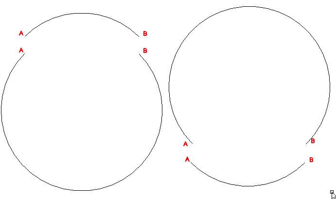 |
| Fig. 3. Four possible arcs of a given radius drawn from A to B. Which one do you want? |
I imagine the choice of storing the tangent of the angle is computation speed. The choice of a quarter of the angle is probably for two reasons:
- Tangent has a period of 180°. Now, if you used the tangent of half the angle subtended, this might appear initially to be sufficient, except that you would not be able to use the sign of the value to decide between CW and CCW since you would need the sign to decide between less than or greater than 180° arcs. You would also have an asymptote get in the way of drawing semi-circles. By storing the tangent of a quarter of the arc subtended, we restrict the the domain to angles which yield a positive tangent and so the sign value can be used for something else. It also avoids data representation limitations until you get close to having a complete circle (at which point, the user should probably consider using a circle). I don't know what the solution technically would be for storing a full circle other than a key value or just not letting the user do that—don't know what happens.
- The diagram above shows some handy interrelationships that allow us to fairly easily calculate the rise (i), the radius, the peak (P), and the center (C). A bit of algebra produces \(r = \frac{u (b^2+1)}{4b}\) and \(i = \frac{b u}{2}\), where \(b\) is the bulge value and \(u\), \(r\) and \(i\) are as in Fig. 2. Calculating \(u\) unfortunately requires a square root, but no trigonometric function calls. Finding C and P involves using \(r\) and \(i\) along with a vector perpendicular to line AB [e.g., \((x,y) \to (-y,x) \), but watch which one gets the negative depending on which way you're turning].
(See Polylines: Radius-Bulge Turnaround for follow up post to this one.)
Wednesday, August 6, 2014
iMaxima and Slime in EMACS
First of all, I am a Windows user. Lots of (probably) very helpful documentation for how to do this is not directly applicable to my setup, because I am not a Linux user. Bummer. That being said, it worked out in the end.
If you just want to hurry up and try Common Lisp in a REPL, then try Lispbox.
I recently set out to do two things:
Watch Installing Common Lisp, Emacs, Slime & Quicklisp: It's a demo of installing EMACS with SBCL, Quicklisp, and Slime.
iMaxima
Visit the main site for iMaxima to see what it's about. It also has a section for installation instructions. Most of what you need to know is on that website. Below are details from my own setup and additional research that helped me get the system up and running on my computer.
After you have EMACS setup and have decided your HOME folder (see here), run EMACS to let it create a ".emacs.d" folder. Then create or edit the file init.el (el means EMACS Lisp, I believe). Here is my entire init.el (largely excepting comments), which includes commands for a REPL with SBCL and iMaxima (separately):
Size of TeX output can be modified using (setq imaxima-fnt-size "xxxx"), where xxxx is one of small, normalsize, large, Large, LARGE, huge, or Huge. Also, by viewing the imaxima.el file, you can see a number of other options that are available to you.
To understand what's happening a bit better, it helps to know a few variables.
If you just want to hurry up and try Common Lisp in a REPL, then try Lispbox.
I recently set out to do two things:
- Get EMACS to run Slime (with any Common Lisp implementation)
- Get EMACS to run iMaxima
Watch Installing Common Lisp, Emacs, Slime & Quicklisp: It's a demo of installing EMACS with SBCL, Quicklisp, and Slime.
- The primary hangup I was having until I saw this video is that I was trying to find a way to get EMACS to do something that I was supposed to do from within a running instance of a selected Common Lisp implementation. In other words, if you want to use CCL in EMACS using Slime, you should run CCL in a cmd window and use that REPL. Like many solutions, it's totally obvious when it is shown to you, which is why you may have trouble finding explicit statements about this.
- If you want to see a few of the basic environment variable modifications in slow motion (as it were), see here.
To start slime, I launch EMACS and then type ALT-X slime ENTER.
Visit the main site for iMaxima to see what it's about. It also has a section for installation instructions. Most of what you need to know is on that website. Below are details from my own setup and additional research that helped me get the system up and running on my computer.
After you have EMACS setup and have decided your HOME folder (see here), run EMACS to let it create a ".emacs.d" folder. Then create or edit the file init.el (el means EMACS Lisp, I believe). Here is my entire init.el (largely excepting comments), which includes commands for a REPL with SBCL and iMaxima (separately):
Size of TeX output can be modified using (setq imaxima-fnt-size "xxxx"), where xxxx is one of small, normalsize, large, Large, LARGE, huge, or Huge. Also, by viewing the imaxima.el file, you can see a number of other options that are available to you.
To understand what's happening a bit better, it helps to know a few variables.
- Go to your scratch buffer in EMACS.
- Type inferior-lisp-program CTRL-j.
- You will get the output "sbcl" if you used my init.el file.
I suggest the scratch buffer because it is important in debugging when you don't have a working setup of anything else. The scratch buffer is available. It runs ELISP, EMACS' own Lisp dialect.
Here are a few other variables you might benefit from looking at:
- load-path
- exec-path
- image-library-alist
I've bolded image-library-alist because it is really helpful to know what file you need to display png files. I snagged the files jpeg62.dll, libpng14-14.dll, and zlib1.dll from a couple of sources and placed them in "C:\Program Files (x86)\emacs-24.3\bin" which is where my "runemacs.exe" is.
- Notably, I got libpng14-14.dll and zlib1.dll from "C:\Program Files (x86)\Inkscape". (You really should try Inkscape, the free SVG editor, anyways.)
- If your image-library-alist has other files in it, you either need to augment your image-library-alist (probably in your init.el file) or find one of the files already in image-library-alist and place it in the load path. You only need to do this for png files (as far as I know) in order to use imaxima.
A command you should try running (still in the scratch buffer) is
(image-type-available-p 'png)
which will return T or NIL depending on whether the file type is available or not, respectively. If you get NIL, it means you don't have one of the files in image-library-alist in your load-path (or perhaps a dependee file is missing?).
Breqn
I had a lot of trouble with the display of the LaTeX even after I had a running imaxima session in EMACS. (Results of evaluations are usually displayed with LaTeX.) The problem stemmed from a missing package: breqn. I installed the mh package from within the MiKTeX Package Manger and it appeared to install fine, but my LaTeX was still not working properly within an imaxima session. The issue appears to have been related to dynamic loading of packages.
Here's what finally shook the problem loose: within TeXnicCenter I started a new project and included the line
\usepackage{breqn}
along with the other \usepackage declarations that were part of that project. When I built the project I was prompted for the installation of the package and the installation appeared to go smoothly. Then I tried imaxima again and the LaTeX output worked.
I had a lot of trouble with the display of the LaTeX even after I had a running imaxima session in EMACS. (Results of evaluations are usually displayed with LaTeX.) The problem stemmed from a missing package: breqn. I installed the mh package from within the MiKTeX Package Manger and it appeared to install fine, but my LaTeX was still not working properly within an imaxima session. The issue appears to have been related to dynamic loading of packages.
Here's what finally shook the problem loose: within TeXnicCenter I started a new project and included the line
\usepackage{breqn}
along with the other \usepackage declarations that were part of that project. When I built the project I was prompted for the installation of the package and the installation appeared to go smoothly. Then I tried imaxima again and the LaTeX output worked.
To start an imaxima session, launch EMACS and then type ALT-x imaxima ENTER.
Piece of cake! :)
Piece of cake! :)
Additional Info (probably not necessary)
I also made another change, and I don't know if it was necessary or not (hopefully not), but while wrestling with something quite different I changed line 14 of maxima-build.lisp (that's "C:\Program Files (x86)\Maxima-5.31.2\share\maxima\5.31.2\src\maxima-build.lisp" on my system). I changed that line to:
I'm still getting a warning message when I load imaxima, although it has yet to prove to be a problem. The warning is:
(lambda (x) ...) quoted with ' rather than with #'
(lambda (x) ...) quoted with ' rather than with #'
I also made another change, and I don't know if it was necessary or not (hopefully not), but while wrestling with something quite different I changed line 14 of maxima-build.lisp (that's "C:\Program Files (x86)\Maxima-5.31.2\share\maxima\5.31.2\src\maxima-build.lisp" on my system). I changed that line to:
(load "C:/Program Files (x86)/Maxima-5.31.2/share/maxima/5.31.2/share/lisp-utils/defsystem.lisp")
This is just an explicit file reference rather than a relative path. (In case you're wondering, I was trying, unsuccessfully, to compile maxima myself. Perhaps another time.)
Tuesday, May 6, 2014
Skew Cut Profiles
I recently was surprised (anew) at what happens when you cut a prism which has a uniform cross-section with a plane which is not orthogonal to the length of the prism. Especially if the plane must be described in terms of two angles. A cross-section through a square prism is (by definition) a square. If you make your cut at an angle, you will get a rectangle if you have a simple angle cut. But if you make your cut not only a miter, but also a bevel you end up with a parallelogram.
The simplest way to visualize this is to imagine a plane that intercepts the prism at a single edge first and has its steepest slope in the direction of the opposite edge:
 The resulting section when viewed in the intersecting plane would be something like this:

where the blue square is the cross-section, the red parallelogram is the intersection of the above described plane through the square prism when viewed in that plane. (A few thought experiments of your own will probably serve you better than any further illustration of this phenomenon I could drum up at the moment.)
It is interesting to see the result in an I-beam shape if you use a 45° miter and 45° bevel:
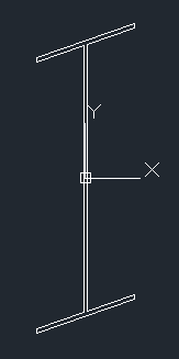
As a matter of where this observation fits into mathematics generally, this is a projective or affine transformation. Such transformations preserve straight lines but they do not, in general, preserve right angles.
Aside: Convex Hulls
The fact that they preserve straight lines is a boon to the would-be-writer of a convex hull algorithm in an arbitrary plane since you can project the 3D coordinates onto a simple 2D plane and use the 2D algorithm (being careful to preserve or restore the other coordinate at the end). If you do so, you should probably choose which set of 2 coordinates to use for the algorithm, based on the direction of the plane. For example, if the normal of the plane has a larger z-coordinate than x- or y-coordinates, then the (x,y) pairs are best to use for the information to run the 2D convex hull algorithm on. There are two reasons to be picky about this:
The simplest way to visualize this is to imagine a plane that intercepts the prism at a single edge first and has its steepest slope in the direction of the opposite edge:
where the blue square is the cross-section, the red parallelogram is the intersection of the above described plane through the square prism when viewed in that plane. (A few thought experiments of your own will probably serve you better than any further illustration of this phenomenon I could drum up at the moment.)
It is interesting to see the result in an I-beam shape if you use a 45° miter and 45° bevel:
As a matter of where this observation fits into mathematics generally, this is a projective or affine transformation. Such transformations preserve straight lines but they do not, in general, preserve right angles.
Aside: Convex Hulls
The fact that they preserve straight lines is a boon to the would-be-writer of a convex hull algorithm in an arbitrary plane since you can project the 3D coordinates onto a simple 2D plane and use the 2D algorithm (being careful to preserve or restore the other coordinate at the end). If you do so, you should probably choose which set of 2 coordinates to use for the algorithm, based on the direction of the plane. For example, if the normal of the plane has a larger z-coordinate than x- or y-coordinates, then the (x,y) pairs are best to use for the information to run the 2D convex hull algorithm on. There are two reasons to be picky about this:
- If the points fed to the routine are in thy yz-plane, you will get incorrect results (if you assumed the (x,y) coordinates should always be used).
- It may reduce the effect of rounding errors in the calculations (in terms of deciding whether points "near the line" of the hull are inside or part of the hull).
(I have lost the original code I used for this post, so I omit references to it now.)
See the Maxima project for download information for Maxima.
Saturday, February 1, 2014
Round 'em up!
Over the past several months I have been dabbling in Common Lisp (LISt Processing language). Lisp, I think, is the ugly duckling of the programming languages. The facetious "Lost In Stupid Parentheses" seems more apt as an acronym.
My first encounter with this ungainly language (Lisp) was in AutoLisp (and Visual Lisp). I was on a hiatus from programming regularly and discovered this immediately discouraging language that was the "easiest" way to interact with AutoCAD programmatically. (I don't consider AutoCAD scripts to be programming, though I would still include them under the more general category automation.) I did not make much headway at that time and it frankly amazes me that any non-programmer will step up to the challenge and learn it.
But then there was Maxima. I was happy with Maxima as a free computer algebra system. But in the documentation I found the spectre of Lisp. Specifically, Common Lisp. The computations in Maxima are all in Lisp (though there is probably some non-Lisp they use to glue together a Windows interface for Maxima). Maxima itself supports a fairly robust set of programming constructs as far as doing calculations are concerned.
My first encounter with this ungainly language (Lisp) was in AutoLisp (and Visual Lisp). I was on a hiatus from programming regularly and discovered this immediately discouraging language that was the "easiest" way to interact with AutoCAD programmatically. (I don't consider AutoCAD scripts to be programming, though I would still include them under the more general category automation.) I did not make much headway at that time and it frankly amazes me that any non-programmer will step up to the challenge and learn it.
But then there was Maxima. I was happy with Maxima as a free computer algebra system. But in the documentation I found the spectre of Lisp. Specifically, Common Lisp. The computations in Maxima are all in Lisp (though there is probably some non-Lisp they use to glue together a Windows interface for Maxima). Maxima itself supports a fairly robust set of programming constructs as far as doing calculations are concerned.
- Input/output from files
- Controlled loops
- if-then-else
- functions
- plotting (via gnuplot—included in standard installs)
- formatted output
- nice math notation display
- export to latex or image
Maxima is built on top of Lisp and you really have all the abilities of Lisp in Maxima (if you know how to get at them). But, being as I am, always in search of a better way of doing something, I am also concerned with whether a technology built on top of another is "hiding" some of the features of the underlying technology. Perhaps hiding isn't exactly the right way to put it, but learning Lisp is a paradigm shift from most other (Algol-like) programming languages I was familiar with, while on the other hand, learning Maxima didn't take me through that paradigm shift.
The two most interesting features of Lisp to me are the emphasis on function references and macros. But they both help you to do the same thing: reduce the repetition in your code. Mind you, they serve this end in very different ways.
When I wanted to implement Jarvis's march [1, p. 955] to encircle a list of points in a "convex hull" it was particularly the function referencing that made the implementation of the code fairly simple.
 |
| Fig 1. The red lines join together the red + signs which indicate the convex hull for these points. |
The general idea of Jarvis's march is you find an outside point to start from and then keep picking the next point so that you never have to switch directions as you walk around. I started at the left most point. In the event of a tie, I choose the lower of these. (That would place us at about (0.1, 15.0).) I decided to walk around the points in a counter-clockwise direction. To decide which point comes next, I need to find the point which requires the right-most turn. So I begin by choosing the first of the remaining points (in whatever order I received them). I go through the remaining points and test whether I would need to make a right turn or left turn to point toward them (from my vantage point on the starting point of the hull chosen at my first step). If it is a right turn, then I have a new winner which replaces the first and I continue moving forward to the points not yet checked. The algorithm is really a repeated application of a maximum function where maximum is defined according to a different function than normal. What I need are predicate functions which define the rules for choosing a winner (a "maximum") and a routine to separate the winner from the remaining points that can accept a predicate function as a parameter. Here's the code for, remove-winner:
The idea of remove-winner is to use the test function (supplied by the caller) to determine whether the next item is "better" than the current winner. If you passed in the function < (using the syntax #'<) you would get the smallest value in the list (provided it was a list of numbers). Notice the thought process in this function is not just to find the max and return it, but rather to produce a list which includes the "winner" and the rest of the values (that didn't win) separately. We don't just need to know the winner, we need to separate the winner from the rest.
When we get to the convex-hull routine, we can use the same routine (remove-winner) using two different tests: one to find the initial element and another to find the successive elements.
The idea of remove-winner is to use the test function (supplied by the caller) to determine whether the next item is "better" than the current winner. If you passed in the function < (using the syntax #'<) you would get the smallest value in the list (provided it was a list of numbers). Notice the thought process in this function is not just to find the max and return it, but rather to produce a list which includes the "winner" and the rest of the values (that didn't win) separately. We don't just need to know the winner, we need to separate the winner from the rest.
When we get to the convex-hull routine, we can use the same routine (remove-winner) using two different tests: one to find the initial element and another to find the successive elements.
The first occasion we use remove-winner, the function is of the same sort we would use to perform a two key sort. In the main body of the routine, we have a more interesting function which accepts two points, calculates their direction vectors (using the current head node of the hull as the origin) and decides whether the second is a right turn away from the first, in which case it declares the second to be the (current) winner.
Can you do this [abstract the predicate] in other languages? Yes. In many other languages you could implement the routine substantially like this. But the key is this: would you ever think to do it this way if you were using VB.NET or C# or C++? Maybe. But not because of your experience with those languages, but because of your experiences with Lisp or F# or other languages which feature a functional style of programming.
Fig. 1 was produced from running a small bit of Maxima code which loads some routines from a separate package written in Lisp (including the above routines). You can download both files to try them out:
You will need to have Maxima installed to try this example out.
Sources:
- Cormen, T.H., Leiserson, C.E., Rivest, R.L., & Stein, C., Introduction to Algorithms, Second Ed., McGraw-Hill Book Company / The MIT Press, 2001.
Subscribe to:
Posts (Atom)