Finding Frequency Fourier Style

Last week, I had a look at the FFT module in Maxima and it was fun times. I was a little disappointed at the interpolated result for the frequency when analyzing the results of the FFT of the 440 Hz waveform. Mind you, if the application is to find a nearest note frequency and, being a human with an at least average sense of musical perception, you already know you're hearing notes that sound like 12 semitones per octave (exclusive counting, i.e., C up to B), then you can coerce the results to the nearest value of  \((440) 2^{i/12}\), for \(i\) over integers. If you don't intend to get any deeper than determining the major pitches, then this is fine. (Could get more tricky if the whole thing is internally shift tuned—everything a half of a semitone flat, but internally tuned, but then maybe you could create a filter to catch that case and accordingly shift your frequency base from 440 to something else that models the sound better.)

We got close enough last time for goal 1 (find the basic notes), but still, I wondered whether I could get closer to the true frequency than last time. I also thought I should use a different example frequency so nobody gets the wrong idea that this is somehow only good for integer frequencies. (Integers are discrete, but discreteness goes beyond just integers.)

So, let's use \((440)  2^{1/12}\) or approximately 466.16 Hz.

load(fft); wave(amp, freq, t) := amp*sin(2*float(%pi)*freq*t); sampleRate: 44100.0$ timeStep: 1/sampleRate$ N: 2^14; inputFFT: makelist(wave(40, 440*2^(1/12), t*timeStep), t, 1, N)$ transformed: real_fft(inputFFT)$ wxplot2d([discrete, makelist(i*sampleRate/N, i, 1, 200), firstn(map(lambda([u], abs(u)), transformed), 200)]);

Fig. 1. Frequency of 466.16 Hz.

wxplot2d([discrete, makelist((i-1)*sampleRate/N, i, 170, 180), map(lambda([u], abs(realpart(u))), firstn(rest(transformed, 169),11))]);

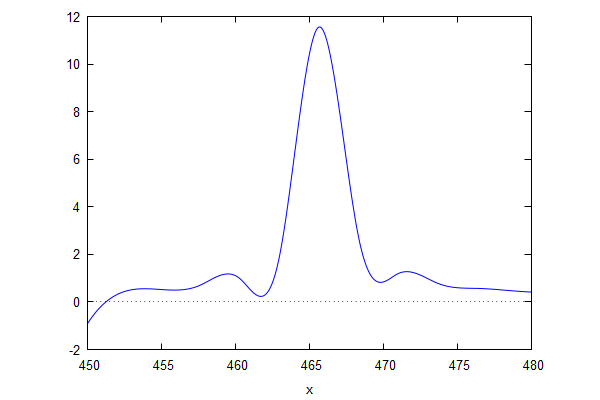
Fig. 2. Zooming in a little closer on the points.

So, let's take these same points and try a cubic spline.

load("interpol")$ f: cspline(map(lambda([f,a], [f, a]), makelist((i-1)*sampleRate/N, i, 170, 180), map(lambda([u], abs(realpart(u))), firstn(rest(transformed, 169),11)))); wxplot2d(f, [x, 450, 480]);

Fig. 3. Cubic spline view of things. Still looks fake. But less fake in the middle.

The cubic spline is helpfully printed out with characteristic functions which are mainly readable. I pick out the one that has the interval of concern, namely, 0.5264689995542815*x^3-738.1894409400452*x^2+345013.3968874384*x-5.374983574143041*10^7. We can use differentiation to find the location of the maximum value.

findMax: 0.5264689995542815*x^3-738.1894409400452*x^2+345013.3968874384*x-5.374983574143041*10^7; diff(findMax, x); float(solve(diff(findMax, x)=0, [x]));  

Which gives roots of [x=465.6995765525049,x=469.0682718425062]. Clearly 465.7 is the one we want. We're not any closer than we were last time using linear interpolation, although the general appearance of the graph looks more realistic and we did include another bit of the Maxima library.

FFT - Local Symmetry Inferred Peak

As I was thinking about the previous post, I thought there might be a way to estimate the location of the peak. That is, to find the location in between the discrete data points where the peak probably occurs. 

I tried using realpart and imagpart and abs to see the differences and it seemed like realpart gives me the best view of the relative amplitudes when there are multiple frequencies involved. I also decided to apply an index shift since that seems to match the frequency better although I'm not satisfied with it technically yet.

Let's zoom in on the location of one of the peaks and see what it looks like:

wxplot2d([discrete, makelist((i-1)*sampleRate/N, i, 160, 170), map(lambda([u], abs(realpart(u))), firstn(rest(transformed, 159),11))]);

Fig. 1. Looks like we should be able to make a better guess than just picking one of the points.

Here are the actual points as frequency, absolute, real part value pairs:

[[427.972412109375,1.373307119161833],[430.6640625,1.783783923237471],[433.355712890625,2.525090138349324],[436.04736328125,4.273342049313825],[438.739013671875,13.47741003943344],[441.4306640625,11.94536977902466],[444.122314453125,4.166745114303215],[446.81396484375,2.532438127248608],[449.505615234375,1.822956914133206],[452.197265625,1.426082632315385],[454.888916015625,1.172306075942115]]

For a first crack at it, we might try linear interpolation on the two pairs of points on either side of the gap that contains the peak. Based on the Wikipedia article of the continuous version, we are certainly deviating from the shape of the real thing. Dauntless we press on to see what we get, because maybe we can live with a slight improvement that we know isn't perfect.

So, here we go do linear interpolation and find the line intersection using Maxima.

Line(A, B) := [x, y] . [A[2]-B[2], B[1]-A[1]] = [A[2]-B[2], B[1]-A[1]] . A; float(solve([ Line([436.04736328125,4.273342049313825],[438.739013671875,13.47741003943344]), Line([441.4306640625,11.94536977902466],[444.122314453125,4.166745114303215])], [x, y]));

[[x=439.729058165623,y=16.86285595968834]]

Let's put that point in the middle and see what it looks like:

revised: [[427.972412109375,1.373307119161833],[430.6640625,1.783783923237471],[433.355712890625,2.525090138349324], [436.04736328125,4.273342049313825],[438.739013671875,13.47741003943344], [439.729058165623,16.86285595968834], [441.4306640625,11.94536977902466],[444.122314453125,4.166745114303215], [446.81396484375,2.532438127248608],[449.505615234375,1.822956914133206],[452.197265625,1.426082632315385],[454.888916015625,1.172306075942115]]$ wxplot2d([discrete, revised]); 

Fig. 2. Hmm, closer, but looks kinda fake to me.

Somewhat predictably, this looks as fake as it really is. I think this graph makes it just how clear that linear interpolation is slightly bogus here. Not completely bogus though, it got us closer, right? So, we've ended up on the left side of the true peak which we know should happen exactly at 440 Hz. Why? The slope on the right side of the true peak is further away from the peak and therefore has a lower (absolute) slope value—it is less steep than it would be if it was closer to the peak. This is the weakness of linear interpolating this. We will end up closer to the higher of the two near-peak points than we should.

To get closer, we might want to try a different type of interpolation. Maybe a cubic spline?