Using CLSQL in LispWorks 8 (x64)

A few modifications are needed to use CLSQL in LispWorks 8.0. The core changes needed are in ...\quicklisp\dists\quicklisp\software\clsql-20210228-git\uffi\clsql-uffi.lisp. I changed the returning clauses in each of the following (and the function names for #-windows conditions):

#-windows

(uffi:def-function ("_strtoui64" c-strtoull)

    ((str (* :unsigned-char))

     (endptr (* :unsigned-char))

     (radix :int))

  :returning :uint64)

#-windows

(uffi:def-function ("_strtoi64" c-strtoll)

    ((str (* :unsigned-char))

     (endptr (* :unsigned-char))

     (radix :int))

  :returning :int64)

#+windows

(uffi:def-function ("_strtoui64" c-strtoull)

    ((str (* :unsigned-char))

     (endptr (* :unsigned-char))

     (radix :int))

  :returning :uint64)

#+windows

(uffi:def-function ("_strtoi64" c-strtoll)

    ((str (* :unsigned-char))

     (endptr (* :unsigned-char))

     (radix :int))

  :returning :int64)

LispWorks didn't know what to do with the :unsigned-long-long.

Two other things to try to make sure you are ready to move forward with your databases. If you are using SQLite3 or MySQL, you will need to locate the required dlls (or download them). Use 

(push (pathname "C:/path/to/x64") 

      clsql::*FOREIGN-LIBRARY-SEARCH-PATHS*)

to allow finding the paths to the dlls. Do this for each of the required dlls.

Each type of database can be loaded according to Database Back-ends. For example, SQLite3:

    (asdf:operate 'asdf:load-op 'clsql-sqlite3)

For an asd file that needs SQLite3, this is what I'm currently using after a call to (ql:quickload :clsql) before defsystem:

(let ((sqlite-path (truename "~/common-lisp/sql/x64"))) (unless (member sqlite-path clsql::*FOREIGN-LIBRARY-SEARCH-PATHS*) (push sqlite-path clsql::*FOREIGN-LIBRARY-SEARCH-PATHS*))) (asdf:operate 'asdf:load-op 'clsql-sqlite3)

After attempting to use the create-view-from-class function and finding that it created tables without foreign keys, I decided to use a simple SQL create script. It appears that execute-command only executes the first SQL statement, so it is necessary to split on the semi-colon (;) and then run each statement in sequence. (I am skipping the last "statement" in my results because my script has some gobble-dee-gook at the end.)

(defun create-project-database (db) (let* ((create-script (slurp (truename "~/common-lisp/project/data/create script.sql"))) (scripts (mapcar #'(lambda (u) (concatenate 'string u ";")) (split-any create-script #\;)))) (setf scripts (subseq scripts 0 (1- (length scripts)))) (loop for s in scripts do (execute-command s :database db)) db))

FFT Parabolic Interpolation

Someone at the Numerix-DSP blog made the reasonable suggestion of interpolating the results of an FFT using a parabola. I did some experimenting with this method and found that it was not any worse than my other methods and it seemed less likely to turn out spurious results.

I've moved out the Maxima domain with my calculations and into Common Lisp, but to create the calculation for the parabolic interpolation, Maxima was of some help. First, we define a function for taking three points, and producing the parabola that is defined by that. 

PolySolve(A, B, C) := block([polyForm, eqn1, eqn2, eqn3], polyForm: a*x^2 + b*x + c = y, eqn1: subst([x=A[1],y=A[2]], polyForm), eqn2: subst([x=B[1],y=B[2]], polyForm), eqn3: subst([x=C[1],y=C[2]], polyForm), subst(solve([eqn1, eqn2, eqn3],[a,b,c]), polyForm) );

Then we will solve for it. We make the observation that the shape of the parabola is the same regardless of shifting it left or right along the x-axis (or index axis, which corresponds to the frequency axis when we multiply by sampling rate). This being the case, we have no need to supply the final indices but can consider our middle point as index 0, the point before it as index -1 and the point after it as index 1. This simplifies the calculation so that we can find the location of the peak relative to the index we are examining and apply the results of this calculation to it. Time to pull in some grade 12 math and differentiate that parabola and find the vertex (see Fig. 1).

Fig. 1. The green dot is approximately where the vertex of this parabola is. The result of this calculation would have x as slightly positive.

poly: PolySolve([-1,y0],[0,y1],[1,y2]); ratsimp(poly); df: diff(poly, x); freq: solve(df, [x]); \[\frac{{{x}^{2}}\, \left( \mathit{y2}-2 \mathit{y1}+\mathit{y0}\right) }{2}-\frac{x\, \left( \mathit{y0}-\mathit{y2}\right) }{2}+\mathit{y1}=y\] \[\frac{\left( {{x}^{2}}+x\right) \, \mathit{y2}+\left( 2-2 {{x}^{2}}\right) \, \mathit{y1}+\left( {{x}^{2}}-x\right) \, \mathit{y0}}{2}=y\] \[x\, \left( \mathit{y2}-2 \mathit{y1}+\mathit{y0}\right) -\frac{\mathit{y0}-\mathit{y2}}{2}=0\] \[[x=-\frac{\mathit{y2}-\mathit{y0}}{2 \mathit{y2}-4 \mathit{y1}+2 \mathit{y0}}]\]

On the basis of this we can produce a common lisp function to perform this calculation.

(defun parabola-peak-frequency (y0 y1 y2) (let* ((y2-y0 (- y0 y2)) (denom (+ (* 2 y2) (* -4 y1) (* 2 y0))) (x (/ y2-y0 denom)) (x^2 (* x x)) (amp (/ (+ (* (+ x^2 x) y2) (* 2 (- 1 x^2) y1) (* (- x^2 x) y0)) 2))) (list x amp)))

Note that if the peak is to the left of our high point, we will get a negative x value and if it is to the right, a positive value. It will be on the interval \((-1, 1)\). Some code that goes through the results of an FFT and takes the absolute value as in our previous work and finds local peaks is all we need now. Where there is a local peak of consecutive absolute values \(a\), \(b\), and \(c\) such that \(a, c < b\), do some interpolation using parabola-peak-frequency to get an interpolated amplitude and an index adjustment for the frequency index. Then the calculation for the the frequency becomes

\[(o + x) s/N\]

where o is the index of \(b\), x is the result from parabola-peak-frequency, s is the sample rate, and \(N \)is the length of elements in the FFT.

Now, maybe we can start applying some math to some real world problems, like, um, Mozart's Piano Concerto No. 13, movement II? Maybe just a snatch within the first second of it for now. 

Fig. 2. Mozart, anyone?

A general outline on how to proceed with this is to identify all of the local peaks, take the top K highest amplitude data points, interpolate those using the parabolic interpolation above, apply pitch correction (if desired) and midi note calculation. This doesn't address determining pitch durations. Another interesting problem is to try to guess which lower peaks are harmonics of lower pitches. These, and probably other confounding problems, yet await.

SQLite Bulk Insert

I was trying to insert a lot of records into an SQLite database and it was taking a long time. Lots amounted to over 137000 in one table. It was taking hours to complete. I decided it must be possible to do the insertion faster with some dynamic SQL. The approach was simple and probably lends itself to some basic abstraction, but I didn't go that far. I could probably use reflection to remove some of the icky repetitive code in it, but this was ok for my immediate needs.

First up, a basic abstract class to inherit. I include some basic convenience functions in it although it might not be great style.

public abstract class bulksert { public abstract string ValueTuple(); public abstract string TablePrefix(); public static string QuotedString(string s) { return "'" + s.Replace("'", "''") + "'"; } public static string NullOrQuoted(string s) { if (s == null) return "null"; else return QuotedString(s); } public static string NullOrNumber(int? i) { if (i.HasValue) return i.Value.ToString(); else return "null"; } public static string NullOrDate(DateTime? dt) { if (dt.HasValue) return QuotedString(dt.Value.ToString("yyyy-mm-dd HH:MM")); else return "null"; } public static string NullOrBit(bool? bit) { if (bit.HasValue) { if (bit.Value) return "1"; else return "0"; } else return "null"; } }

Next up, inherit the class in the table definitions you will use.

public class Versification : bulksert { public Versification() { } public Versification(GreekMorphNTRow grow) { BookIndex = grow.Book; Chapter = grow.Chapter; Verse = grow.Verse; WordIndex = grow.WordIndex; Text = grow.Text; Word = grow.Word; NormalizedWord = grow.Lemma; if (grow.AnalyticId.HasValue) AnalyticId = grow.AnalyticId.Value; } [PrimaryKey, AutoIncrement] public int Id { get; set; } public int BookIndex { get; set; } public int Chapter { get; set; } public int Verse { get; set; } public int WordIndex { get; set; } [MaxLength(50)] public string Text { get; set; } [MaxLength(50)] public string Word { get; set; } [MaxLength(50)] public string NormalizedWord { get; set; } [ForeignKey(typeof(AnalyticLookup))] public int AnalyticId { get; set; } public override string TablePrefix() { return "insert into Versification (BookIndex, Chapter, Verse, WordIndex, Text, Word, NormalizedWord, AnalyticId) values "; } public override string ValueTuple() { StringBuilder sb = new StringBuilder(); sb.Append("("); sb.Append(NullOrNumber(BookIndex)); sb.Append(","); sb.Append(NullOrNumber(Chapter)); sb.Append(","); sb.Append(NullOrNumber(Verse)); sb.Append(","); sb.Append(NullOrNumber(WordIndex)); sb.Append(","); sb.Append(NullOrQuoted(Text)); sb.Append(","); sb.Append(NullOrQuoted(Word)); sb.Append(","); sb.Append(NullOrQuoted(NormalizedWord)); sb.Append(","); sb.Append(NullOrNumber(AnalyticId)); sb.Append(")"); return sb.ToString(); } }  

Here are the two main reuseable routines that save a lot of time doing the inserts. They assume all the records are really of the same type, which is the most common application for a bulk insert. I don't know of any reason to make the inserts accommodate multiple types, but it would be possible to apply a partition at the start if you have an application for that. 

  public Task<int> Bulksert(IEnumerable<bulksert> bulks) { StringBuilder sb = new StringBuilder(); string prefix = bulks.First().TablePrefix(); sb.AppendLine(prefix); sb.Append(bulks.First().ValueTuple()); foreach(var b in bulks.Skip(1)) { sb.AppendLine(","); sb.Append(b.ValueTuple()); } sb.AppendLine(";"); return database.ExecuteAsync(sb.ToString()); } public Task<int> Bulksert(IEnumerable<bulksert> bulks, int clusterSize) { var cluster = bulks.Take(clusterSize); var remaining = bulks.Skip(clusterSize); var InitialTask = Bulksert(cluster); if (remaining.FirstOrDefault() == null) return InitialTask; else return InitialTask.ContinueWith(ti => Bulksert(remaining, clusterSize)).Unwrap(); }

Note that the syntax for these inserts is very specific to SQLite.

What's in Your Vocabulary Deck?

I am something of a student of New Testament Greek and made my beginnings a few years ago with Mounce's Basics of Biblical Greek. Along with the text book was a flash card program called FlashWorks, and it is a solid way to learn your vocab. The vocab was indexed with frequency and chapter and user level difficulty (based on how often you answered correctly) which was almost all that I wanted to help me keep track of which words I should be working on. 

There was one thing that I felt was missing, though I wasn't sure how to define it or to decide what could be done about it. Something like, "how do I get a balanced randomness to my vocab selection if I only want to do a few right now?"

I don't want to randomly select 10 words from out of 500 words. I won't get much repetition if I do that every day. On the other hand, if I only focus on the most frequent, hard words, then I repeat them every day, then the risk might be that I "cram" them and don't really get them into long term memory. So, maybe the thing to do is to start with a selection of 30 words that are the most difficult/frequent words and randomly select 10 from that list. I call it a "pool factor". The pool factor in that case, would be 3. Make a selection of the most difficult, frequent words up to 30 long (and include a random sorting factor in case there are contenders for the last spots in the 30) and then randomly select 10 out of the 30.

The 30 words are a kind of "working set" that I am working toward mastering, although, I don't need to specifically decide on them, they get selected based on criteria. I do 10 words today out of those 30. As I do the daily work, some of those 30 words drop out because I got them right a bunch of time and new words enter the selection of 30.

The next issue is to decide what is meant by hardest, frequent words. If I use a score that starts high for words that have never been marked correct, then I can do a descending sort on score, then by frequency. The whole deck will start at the highest score and initially I am getting the most frequent words. In order to prevent words from disappearing from this set too soon, keep track of not just a score, but the number of times marked correct. Only decrease the score after after getting the word right correct, say, 3 consecutive times. (Since the score of a word doesn't change until you have reached a level of mastery with it, you don't run into the scenario of interchanging sets of words that you then never master.)

Note that you can probably apply this strategy to other types of vocabulary that don't reference a fixed body of literature, but you have to come up with some kind of importance rating on each word in your database that serves the same purpose as the frequency field here.

The code below belongs to a C# project of mine that is using SQLiteAsyncConnection with some fields that are still missing data (hence, ifnull):

        public Task<List<Vocab>> GetNRandomHardFrequent(int numberOfWords, double poolFactor)

        {

            int PoolSize = Convert.ToInt32(numberOfWords * poolFactor);

            Random rand = new Random();

            string query = @"

                    select 

                        sub.*

                    from

                        (select 

                            v.*

                        from

                            Vocab v

                        order by

                            ifnull(v.score, 0) desc, ifnull(v.frequency, 0) desc, RANDOM()

                        limit ?) sub

                    order by

                        RANDOM()

                    limit ?;";

                        

            var words = database.QueryAsync<Vocab>(query, PoolSize, numberOfWords); 

            return words;

        }

FFT - DIY

There's more than enough information freely available to enable you to make your own FFT. You can review the pseudo-code from Wikipedia to make it yourself. I have been raving about this bit of Mathematics for several posts now. I knew that the FFT (\(O(N \log {N})\)) was much faster than computing the DFT (\(O(N^2)\)) from the definition. But how much faster is it really when you compare the methods with realistic data sets? Sorting algorithms have this difference but with small data sets (even thousands of points) like most of us work with, it doesn't matter that much.

Whenever you go about to make something that is somewhat complex, you want a more than casual check to verify that you have the right answer. One way of doing this is to create a simple method that doesn't have any complexities related to speeding up the algorithm or computation in it and use it as a reference against the more complex method you want to test. You can also find the results of someone else's work and compare against that.

I made both a DFT and FFT (dit-fft2) method and tried them out. I noticed while testing these out that I get results that agree with each other, but they differ from the results I got in Maxima in two ways: 1) the overall values appear to be factored in the Maxima FFT and there was a difference in sign on the imaginary component. I suspect Maxima is normalizing by length and using positive roots of unity instead of negative roots of unity. (Signal processing people like negative roots of unity and some other people like positive roots of unity. Go figure.) To test for consistency I used create-test-data for a small data set of 32 points and applied both dft and dit-fft2 to it. They come out the same, so I'm reasonably certain that the calculation was done correctly. 

Next, I tried a larger data set, \(2^{14}\) data points. With a sampling rate of 44100 Hz, this is about 0.37s worth of PCM data. The DFT function ran in 2:41 min and the dit-fft2 function ran in 0.125s. Even at 0.125s, that is a long time to process if you have much data to churn through. A brief review of the dit-fft2 function will show that there is a lot of data copying involved in this version and so methods which avoid the need to copy data around by using an indexing scheme are likely to increase performance significantly.

Enough already—code me!

(defparameter *sample-rate* 44100) (defparameter *two-pi* (* 2 pi)) (defun waveform (amplitude frequency) (let ((omega (* *two-pi* frequency))) #'(lambda(time) (* amplitude (sin (* omega time)))))) (defun create-test-data (amplitude frequency sample-rate N) (let* ((w (waveform amplitude frequency)) (time-step (/ 1 sample-rate)) (arr (make-array N :initial-element 0.0))) (loop for i from 0 to (1- N) do (setf (aref arr i) (funcall w (* i time-step)))) arr)) (defun dft (pcm) (let* ((Num (length pcm)) (res (make-array Num :initial-element 0.0))) (loop for k from 0 to (1- Num) do (setf (aref res k) (loop for n from 0 to (1- Num) sum (* (aref pcm n) (exp (/ (* -1 #C(0 1) *two-pi* k n) Num)))))) res)) (defun arrayify (li N) (make-array N :initial-contents li)) (defun dit-fft2-wh (x N) (cond ((= N 1) x) (t (let* ((hN (/ N 2)) (x0-inp (arrayify (loop for i from 0 to (1- N) by 2 collect (aref x i)) hN)) (evens (dit-fft2-wh x0-inp hN)) (xn_2-inp (arrayify (loop for i from 1 to (1- N) by 2 collect (aref x i)) hN)) (odds (dit-fft2-wh xn_2-inp hN)) (res (make-array N :initial-element 0))) (loop for k from 0 to (1- hN) for k+N_2 = (+ k hN) for e2pi = (exp (/ (* -1 *two-pi* #C(0 1) k) N)) for e2pix = (* e2pi (aref odds k)) for temp = (aref evens k) do (setf (aref res k) (+ temp e2pix) (aref res k+N_2) (- temp e2pix))) res)))) (defun dit-fft2 (pcm) (let* ((length-to-transform (expt 2 (floor (/ (log (length pcm)) (log 2))))) (x (make-array length-to-transform))) (loop for i = 0 then (1+ i) for p across pcm do (setf (aref x i) p)) (dit-fft2-wh x length-to-transform)))

FFT - Revisiting Symmetry

There was something missing in my last post that might have created part of the problem with the results. Although I observe what looked like symmetry, I didn't constrain any of my interpolated results based on that assumption of symmetry. So, I thought to myself, there ought to be a mathematical way to tell my equations that they should assume a symmetrical situation, the way I am expecting it to look. I'm not really sure this is broadly applicable, but my intuition about a sine wave is that it should have some kind of symmetry in the resulting appearance. This seems to be borne out by scattered examples of continuous Fourier transforms.

I'm not yet sure how to use symmetry, to find the value, but I can see a way to evaluate the accuracy of a given guess. Mind you, I only know how to evaluate it by appearance. Let's introduce a little formula I will call the flip formula.

$$F(x, C) = 2 C - x$$

Suppose you choose \(C = 440\), meaning that you are going to treat 440 as the center. So, for example, \(F(439, 440) = 441\) and \(F(441, 440) = 439\). Let's apply the flip function to the data in one of our previous examples and see what it looks like when we assume the center is 440. 

First, here is the graph we had with just a few points near the peak:

Fig. 1. Just the results of the FFT.

Flip(x, freq) := 2*freq - x$ thePoints: [[427.972412109375,1.436293850207828],[430.6640625,1.84470452365816],[433.355712890625,2.584065181382392],[436.04736328125,4.330481956818618],[438.739013671875,13.53281618900214],[441.4306640625,11.89160409385532],[444.122314453125,4.114533847954862],[446.81396484375,2.48170175135288],[449.505615234375,1.773621776595303],[452.197265625,1.378080393261782],[454.888916015625,1.125573209744724]]$ flippedPoints: map(lambda([u], [Flip(u[1], 440),u[2]]), thePoints)$ allPoints: sort(append(thePoints, flippedPoints), lambda([a, b], a[1] <= b[1]))$ wxplot2d([discrete, map(lambda([u], u[1]), allPoints), map(lambda([u], u[2]), allPoints)]); 

 Let's have a look at what it looks like when we use 439.5, 439.8, and 440.

Fig. 2. "Guessing" frequency 439.5 Hz. Sure doesn't look smooth.

Fig. 3. "Guessing" frequency 439.8 Hz. Looks better.

Fig. 4. "Guessing" frequency 440 Hz. Looks about as smooth as we're going to get.

There are some considerable drawbacks to this approach. The biggest one is that I had to look at the results. The second drawback is that I don't have a number to put to these to decide which is better. And this is transformed from one of the simplest types of wave, a sine wave. To evaluate the soundness of the guess, I would need some formula to fit the points to.

Finding Frequency Fourier Style

Last week, I had a look at the FFT module in Maxima and it was fun times. I was a little disappointed at the interpolated result for the frequency when analyzing the results of the FFT of the 440 Hz waveform. Mind you, if the application is to find a nearest note frequency and, being a human with an at least average sense of musical perception, you already know you're hearing notes that sound like 12 semitones per octave (exclusive counting, i.e., C up to B), then you can coerce the results to the nearest value of  \((440) 2^{i/12}\), for \(i\) over integers. If you don't intend to get any deeper than determining the major pitches, then this is fine. (Could get more tricky if the whole thing is internally shift tuned—everything a half of a semitone flat, but internally tuned, but then maybe you could create a filter to catch that case and accordingly shift your frequency base from 440 to something else that models the sound better.)

We got close enough last time for goal 1 (find the basic notes), but still, I wondered whether I could get closer to the true frequency than last time. I also thought I should use a different example frequency so nobody gets the wrong idea that this is somehow only good for integer frequencies. (Integers are discrete, but discreteness goes beyond just integers.)

So, let's use \((440)  2^{1/12}\) or approximately 466.16 Hz.

load(fft); wave(amp, freq, t) := amp*sin(2*float(%pi)*freq*t); sampleRate: 44100.0$ timeStep: 1/sampleRate$ N: 2^14; inputFFT: makelist(wave(40, 440*2^(1/12), t*timeStep), t, 1, N)$ transformed: real_fft(inputFFT)$ wxplot2d([discrete, makelist(i*sampleRate/N, i, 1, 200), firstn(map(lambda([u], abs(u)), transformed), 200)]);

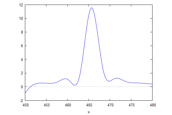
Fig. 1. Frequency of 466.16 Hz.

wxplot2d([discrete, makelist((i-1)*sampleRate/N, i, 170, 180), map(lambda([u], abs(realpart(u))), firstn(rest(transformed, 169),11))]);

Fig. 2. Zooming in a little closer on the points.

So, let's take these same points and try a cubic spline.

load("interpol")$ f: cspline(map(lambda([f,a], [f, a]), makelist((i-1)*sampleRate/N, i, 170, 180), map(lambda([u], abs(realpart(u))), firstn(rest(transformed, 169),11)))); wxplot2d(f, [x, 450, 480]);

Fig. 3. Cubic spline view of things. Still looks fake. But less fake in the middle.

The cubic spline is helpfully printed out with characteristic functions which are mainly readable. I pick out the one that has the interval of concern, namely, 0.5264689995542815*x^3-738.1894409400452*x^2+345013.3968874384*x-5.374983574143041*10^7. We can use differentiation to find the location of the maximum value.

findMax: 0.5264689995542815*x^3-738.1894409400452*x^2+345013.3968874384*x-5.374983574143041*10^7; diff(findMax, x); float(solve(diff(findMax, x)=0, [x]));  

Which gives roots of [x=465.6995765525049,x=469.0682718425062]. Clearly 465.7 is the one we want. We're not any closer than we were last time using linear interpolation, although the general appearance of the graph looks more realistic and we did include another bit of the Maxima library.

FFT - Local Symmetry Inferred Peak

As I was thinking about the previous post, I thought there might be a way to estimate the location of the peak. That is, to find the location in between the discrete data points where the peak probably occurs. 

I tried using realpart and imagpart and abs to see the differences and it seemed like realpart gives me the best view of the relative amplitudes when there are multiple frequencies involved. I also decided to apply an index shift since that seems to match the frequency better although I'm not satisfied with it technically yet.

Let's zoom in on the location of one of the peaks and see what it looks like:

wxplot2d([discrete, makelist((i-1)*sampleRate/N, i, 160, 170), map(lambda([u], abs(realpart(u))), firstn(rest(transformed, 159),11))]);

Fig. 1. Looks like we should be able to make a better guess than just picking one of the points.

Here are the actual points as frequency, absolute, real part value pairs:

[[427.972412109375,1.373307119161833],[430.6640625,1.783783923237471],[433.355712890625,2.525090138349324],[436.04736328125,4.273342049313825],[438.739013671875,13.47741003943344],[441.4306640625,11.94536977902466],[444.122314453125,4.166745114303215],[446.81396484375,2.532438127248608],[449.505615234375,1.822956914133206],[452.197265625,1.426082632315385],[454.888916015625,1.172306075942115]]

For a first crack at it, we might try linear interpolation on the two pairs of points on either side of the gap that contains the peak. Based on the Wikipedia article of the continuous version, we are certainly deviating from the shape of the real thing. Dauntless we press on to see what we get, because maybe we can live with a slight improvement that we know isn't perfect.

So, here we go do linear interpolation and find the line intersection using Maxima.

Line(A, B) := [x, y] . [A[2]-B[2], B[1]-A[1]] = [A[2]-B[2], B[1]-A[1]] . A; float(solve([ Line([436.04736328125,4.273342049313825],[438.739013671875,13.47741003943344]), Line([441.4306640625,11.94536977902466],[444.122314453125,4.166745114303215])], [x, y]));

[[x=439.729058165623,y=16.86285595968834]]

Let's put that point in the middle and see what it looks like:

revised: [[427.972412109375,1.373307119161833],[430.6640625,1.783783923237471],[433.355712890625,2.525090138349324], [436.04736328125,4.273342049313825],[438.739013671875,13.47741003943344], [439.729058165623,16.86285595968834], [441.4306640625,11.94536977902466],[444.122314453125,4.166745114303215], [446.81396484375,2.532438127248608],[449.505615234375,1.822956914133206],[452.197265625,1.426082632315385],[454.888916015625,1.172306075942115]]$ wxplot2d([discrete, revised]); 

Fig. 2. Hmm, closer, but looks kinda fake to me.

Somewhat predictably, this looks as fake as it really is. I think this graph makes it just how clear that linear interpolation is slightly bogus here. Not completely bogus though, it got us closer, right? So, we've ended up on the left side of the true peak which we know should happen exactly at 440 Hz. Why? The slope on the right side of the true peak is further away from the peak and therefore has a lower (absolute) slope value—it is less steep than it would be if it was closer to the peak. This is the weakness of linear interpolating this. We will end up closer to the higher of the two near-peak points than we should.

To get closer, we might want to try a different type of interpolation. Maybe a cubic spline?

FFT in Maxima

Maxima has a basic fast Fourier transform package called fft. Here's are really basic introduction to using it on music data. We define a basic sine wave form with frequency 440 Hz and amplitude 40 as our input and then run fft on it. The interpretation of the results as frequency depends on coordinating together the sample rate, the total number of samples (N), and the sample index (i).

wave(amp, freq, t) := amp*sin(2*float(%pi)*freq*t); sampleRate: 44100.0$ timeStep: 1/sampleRate$ N: 2^14; inputFFT: makelist(wave(40, 440, t*timeStep), t, 1, N)$ transformed: fft(inputFFT)$ wxplot2d([discrete, makelist(i*sampleRate/N, i, 1, 200), firstn(map(lambda([u], abs(u)), transformed), 200)]);

Fig 1. Looks like about 440 Hz

The thing that most threw me for a loop in trying to make sense of the various sources I read was that the x axis needs to be inferred in order to be comprehensible. I wasn't really clear on what that x-axis was. If you dig into the details of the output numbers, you will find the 164th value, has the maximum value. This implies 164 * 44100 / 2^14 = 441 Hz. So, a bit of error has crept into our interpretation of the result because of the discrete nature of the intermediate result. What this means in theory is that there is a theoretical peak that "should" exist somewhat before the 164th index, but because we aren't working with continuous data, we can't see that peak (at the ~163.47th index 😜--or maybe we should be considering it at the 164.47 "index" and subtract 1, interpreting it as zero based, since the peak is probably between the 164th and 165th index).

If we change the function to have two wave forms at different frequencies (340 Hz and 440 Hz), we get both of these in the result:

Fig. 2. wave(20, 340, t*timeStep) + wave(40, 440, t*timeStep)

Next step, in search of the true peak.

EMACS with Slime on Chromebook

Because of a felt-insufficiency of nerdness in my life, I decided it was high time I get set up to use slime in EMACS on a Chromebook. I have been an EMACS user on Windows, using it for my first experience of Common Lisp development. I now use LispWorks on my Windows machine but if there was a way to do Common Lisp on my Chromebook I thought I would hazard some of my time to learn how to go about it.

First, get Linux on your Chromebook. For newer systems, this is as simple as turning on Linux Beta in the user settings of your Chromebook. I don't know how well this works on older Chromebooks, but I understand there are ways.

With Linux enabled or installed as required, go to the terminal (settings key, type linux or terminal and you should see it) and type sudo apt-get install emacs25. I had to run an update to apt-get for this to work properly (sudo apt-get update). Then I redid the emacs25 install (same command line) and it caught up the parts it missed the first time. 

Similarly, you can install a version of Common Lisp. I chose Steel Bank Common Lisp (sbcl). The command line for that is (perhaps predictably) sudo apt-get install sbcl.

Quicklisp is next. I downloaded it from here. I moved it into my Linux files because it seemed like a good idea off hand, though I'm not sure that it is strictly necessary. Before trying to load this, I checked out the (rather simple) file structure on my Linux system from the terminal perspective. Use the ls command to see the files in the current directory and the cd command to change directory (I'm not a real Linux user, maybe you're not either). Next, I started sbcl by typing it at the command line. This results in bringing you to a command line version of sbcl where you can type Common Lisp commands. We use this to load Quicklisp. I issue the following, pressing enter after each line:

    (load "quicklisp.lisp")

    (quicklisp-quickstart:install)

    (ql:add-to-init-file)

    (ql:quickload "quicklisp-slime-helper")

    (quit)

Now, you need some code added to the the init file, but I didn't see such a file and wasn't sure where to put it. Fortunately, there's a way for EMACS to help you with that. Go into EMACS and type CTRL+x CTRL+f, it will assume you want the home directory and lead you with "~/", and so you add to that emacs.d/init.el and press enter. Or, in EMACSese, that's C-x C-f ~/emacs.d/init.el RET. HT to the Wiki. This will create and open the file for you. 

The code you will want to put in this file is suggested at the end of installing the quicklisp-slime-helper and it is this:

    (load (expand-file-name "~/quicklisp/slime-helper.el"))

      (setq inferior-lisp-program "sbcl")

Paste the code into the file you just opened. Now, be prepared for a "wha?" moment. The shortcut sequence for pasting into EMACS is CTRL+y. Or, C-y as the EMACS users like to say. This will not be your last such moment, but carry on.

You are now prepared to start writing and executing Common Lisp code in EMACS. In the below, C- means press and hold CTRL and M- means press and hold ALT. I do the following sequence as a standard way to get started:

    C-x 3 (gets you set with vertical division--left and right panes. one for code file and one for REPL)

    M-x slime RET (starts the REPL)

Here is the classic video tutorial (HT Baggers) of most of these steps done for Windows that also gives a bit of a flavor of what it is like to use Slime in EMACS for Common Lisp development: Installing Common Lisp, Emacs, Slime & Quicklisp.

CLSQL in LispWorks: Varchar Fields

 I was attempting to use CLSQL in LispWorks and had trouble reading in strings. I could even output the strings using insert, but couldn't read them in properly. I had two main issues that I needed to make changes for (running LispWorks 7.1.2 64-bit running on Windows 10, update, now running version 8.0.1 and this is working).

First, LispWorks didn't like a return type of :unsigned-long-long in "...\quicklisp\software\clsql-20160208-git\uffi\clsql-uffi.lisp". Replace these references to :unsigned-long-long with '(:unsigned :long :long) and then it will compile properly. I can't speak for whether this 100% right and I don't think that any of my current code depends on getting this right. But, it does let me compile.

The next problem was in "...\quicklisp\software\uffi-20180228-git\src\strings.lisp", the function fast-native-to-string. There's two such definitions which are split across different versions of lisp. LispWorks 7.1.2 is in the first such definition and there is a reference to base-char that is specifically used for LispWorks.

Edit: Based on comment below from a reader, the changes to make here are:

• line 500: #+(or (and allegro (not ics)) lispworks4)
• line 513: #+(or (and allegro ics) (and lispworks (not lispworks4)))

You will end up with:

#+(or (and allegro (not ics)) lispworks4) (defun fast-native-to-string (s len) (declare (optimize (speed 3) (space 0) (safety 0) (compilation-speed 0)) (type char-ptr-def s)) (let* ((len (or len (strlen s))) (str (make-string len))) (declare (fixnum len) (type (simple-array #+lispworks base-char #-lispworks (signed-byte 8) (*)) str)) (dotimes (i len str) (setf (aref str i) (uffi:deref-array s '(:array :char) i))))) #+(or (and allegro ics) (and lispworks (not lispworks4))) (defun fast-native-to-string (s len) (declare (optimize (speed 3) (space 0) (safety 0) (compilation-speed 0)) (type char-ptr-def s)) (let* ((len (or len (strlen s))) (str (make-string len))) (dotimes (i len str) (setf (schar str i) (code-char (uffi:deref-array s '(:array :unsigned-byte) i))))))

I made a simple table with data that contains both varchar(50) and nvarchar(50) to test with, defined below. I put (mostly) the same data in each of Name and Name1 to see if there was any difference.

CREATE TABLE [dbo].[TableWithStrings]( [Id] [int] IDENTITY(1,1) NOT NULL, [Name] [varchar](50) NOT NULL, [Name1] [nvarchar](50) NOT NULL, CONSTRAINT [PK_TableWithStrings] PRIMARY KEY CLUSTERED ( [Id] ASC )WITH (PAD_INDEX = OFF, STATISTICS_NORECOMPUTE = OFF, IGNORE_DUP_KEY = OFF, ALLOW_ROW_LOCKS = ON, ALLOW_PAGE_LOCKS = ON) ON [PRIMARY] ) ON [PRIMARY]

Using clsql to get all of the tuples that were entered is as simple as (clsql:query "select Id, Name, Name1 from TableWithStrings").

I'm not able to find who to contact regarding this as I see that the website for the project may have been abandoned (last change on the change list was in Jan 2016, specifically for LispWorks support). I note however, that someone more recently made a change for uffi as the folder name has the date in it suggesting Feb 2018.

BMI Table with Undue Precision

The undue precision will be on my part because this post isn't really about your health, it's about doing a little mathematics. In a spreadsheet, because sometimes it's more fun there.

I have a little spreadsheet with a few examples of interesting formulas in Excel. The thing that is a bit pitiful about it is that it isn't an inline formula but a dependency which makes it hard to copy and paste. I did a piece-meal copy and paste job from here (NIH) into a table. 

If you just want a spreadsheet that does this stuff for you and don't care about my blathering, download it here.

The thing that makes this table a beast is that the general usage requires you to first choose only one row of the table based on your height and then find which two weights you fall between and look up to find the BMIs you are between. And since this is a post about interpolation, you do straight interpolation to get your BMI. So, if I'm 5' - 10 1/4", and I'm dead sure to rights I'm not a 1/4" shorter, how do I proceed to get a more accurate value.

Of course, it is eye-roll worthy to care about such precision when the BMI number is a ballpark notion, anyway. But, from the stand point of data and formulas, can we do it anyway? (And, what might we learn if we do?) Here is what I have right now in all of its glorious ridiculousness:

Fig. 1 - Interpolation on steroids. Or maybe, interpolation without boundaries. Well, ok, interpolation without reason.

The simplest way of combining linear interpolations I could think of was to determine boundaries and look up the corresponding values. So we start with finding the low and high lines, in this case the lines for 70 and 71. Looking up the BMI weight included array formulas on the right hand side of the table that reference the given weight.

On the far right of the table I have formulas like the following in columns AL to AO:

• =MAX(IF(B4:AK4<=B$25,B4:AK4, 0))
• find the largest value in B4:AK4 that is still smaller than the weight in B25
• =MIN(IF(B4:AK4>=B$25,B4:AK4, 100000))
• find the smallest value in B4:AK4 that is still bigger than the weight in B25
• =LOOKUP(AL4, $B4:$AK4, $B$2:$AK$2)
• =LOOKUP(AM4, $B4:$AK4, $B$2:$AK$2)

It is important to use the <ctrl> + <shift> + <enter> key combination to make the first two of these formulas work as this is how you create array formulas out of formulas that are not inherently array based. (Formulas that are expecting ranges by default are inherently array based.) Taking the first formula as an example, the meaning of the syntax is something like this: "For every value in the list  B4:AK4, apply this formula." The formula being applied is the IF.  Anywhere you see B4:AK4 you can read, "any x that is in B4:AK4." If you C#'d this, you have something like:

     (B4:AK4).select(x => if(x < B25, x, 0)).max()

LOOKUP is listed as available for backward compatibility. Sounds like it is not really desired and probably the VLookup and HLookup functions are mostly preferred, but LOOKUP has a leg up on them in one respect. I don't have to modify the layout of my table to accommodate my present purpose. I need the search value to be the current row and the return value to be the top value of a column. If I use HLookup, I need the searched value to be the top row (as far as I can see, at least). If I didn't have LOOKUP, I still have a way, of course. Copy the BMI to the bottom and return the bottom row. To my mind, the design of LOOKUP communicates purpose much more effectively: "Here is what I'm searching--shown first, Here is what I want returned from, respectively to the matching item in the search space." 

The rest is just repeated application of linear interpolation. Do linear interpolation for 70 inches (in my case) and then for 71 inches. Then interpolate between those resulting BMIs to get a final BMI. In some cases I omit denominators and/or calculations where I know the result will give me 1 due to the way the spreadsheet and data set is constructed and so these get simplified out of the formulas.

Cluster / Hierarchical Hashing in Common Lisp

I had some application ideas where I wanted to group data by several keys. Sometimes I care about the hierarchical relationship and sometimes I don't. As an example, let's take my FitNotes exercise data. Here's a few records from way back in the day (I can hardly believe the numbers, ugh...a few years and many pounds ago):

Date	Exercise	Category	Weight (lbs)	Reps
2015-03-10	Deadlift	Back	130	10
2015-03-10	Deadlift	Back	130	10
2015-03-10	Deadlift	Back	130	10
2015-03-10	Chin Up	Back	205	4
2015-03-10	One-Arm Standing Dumbbell Press	Shoulders	25	12
2015-03-10	One-Arm Standing Dumbbell Press	Shoulders	25	12
2015-03-10	One-Arm Standing Dumbbell Press	Shoulders	25	12
2015-03-10	Flat Dumbbell Fly	Chest	30	10
2015-03-10	Flat Dumbbell Fly	Chest	30	10
2015-03-14	Deadlift	Back	135	10

If I wanted to show a history of data and provide the user with the option of seeing a graph of their progress (similar to what the FitNotes application does) or perhaps a list of dates to select from to see the details on that date, then I would group first by Exercise and then by date. Depending on the purpose of the grouping, I might want to group by Category first. But let's go with a graphing application for a particular exercise. I want to group by Exercise and then by date.

I create hash tables at each level except the bottom level where I create a queue. The main thing that interested me here was the setf function, since the syntax bamboozled me the first time I saw in Practical Common Lisp (it's not hard, just different). I ended up not needing it for my current application, but may want it another day. For the kind of data I'm working with you need to use the equal test in order to get your hash tables to work with strings. If you compare (setf get-cluster-hash) with add-to-cluster-hash, you'll notice they are very similar. I was tempted to make add-to-cluster-hash out of the setf and get-cluster-hash functions but realized that that entails evaluating the hashes twice for adding the first record to a cluster-key. There might be a way to eliminate the code duplication, but I gave in to copy-paste-modify. (Please don't hate me.)

(defun make-queue () (let ((li (cons nil nil))) (setf (car li) (cons nil nil)) (setf (cdr li) (car li)) li)) ;; we add to the end and maintain the pointer (defun add-queue (queue item) (setf (cddr queue) (cons item nil)) (setf (cdr queue) (cddr queue)) queue) (defun queue->list (queue) (cdar queue)) (defun (setf get-cluster-hash) (value keys hash) (let* ((f (first keys)) (r (rest keys))) (cond ((null f) nil) ((null r) (setf (gethash f hash) value)) (t (let* ((f-hash (gethash f hash))) (unless f-hash (setf f-hash (make-hash-table :test #'equal)) (setf (gethash f hash) f-hash)) (setf (get-cluster-hash r f-hash) value)))))) (defun get-cluster-hash (keys hash) (loop for k in keys for k-hash = (gethash k hash) then (gethash k k-hash) while k-hash finally (return k-hash))) (defun add-to-cluster-hash (keys hash value) (let* ((f (first keys)) (r (rest keys))) (cond ((null f) nil) ((null r) (let ((q (gethash f hash))) (if q (add-queue q value) (let ((nq (make-queue))) (add-queue nq value) (setf (gethash f hash) nq))))) (t (let* ((f-hash (gethash f hash))) (unless f-hash (setf f-hash (make-hash-table :test #'equal)) (setf (gethash f hash) f-hash)) (add-to-cluster-hash r f-hash value))))))

Here is a simple demonstration REPL session with some of these functions:

UTIL 231 > (setf h (make-hash-table :test #'equal)) #<equal Hash Table{0} 200A075F> UTIL 232 > (add-to-cluster-hash (list "deadlift" "2015-03-10") h (list 130 10)) ((NIL (130 10)) (130 10)) UTIL 233 > (add-to-cluster-hash (list "deadlift" "2015-03-10") h (list 130 10)) ((NIL (130 10) (130 10)) (130 10)) UTIL 234 > (add-to-cluster-hash (list "deadlift" "2015-03-10") h (list 130 10)) ((NIL (130 10) (130 10) (130 10)) (130 10)) UTIL 235 > (get-cluster-hash (list "deadlift" "2015-03-10") h) ((NIL (130 10) (130 10) (130 10)) (130 10)) UTIL 236 > (queue->list (get-cluster-hash (list "deadlift" "2015-03-10") h)) ((130 10) (130 10) (130 10))

Since I have the data of interest in a CSV file exported from FitNotes, I can just read every line of the CSV file and use add-to-cluster-hash for each line, thus grouping my data without loosing the order of the items for each (exercise, date), and all without thinking much about the details of the data structure used to do the grouping.

Macro Expansion Time: Connection Strings

Connection strings bother me. I'm not saying that aren't a good solution or that they shouldn't be, but I don't like having to look up special values to fill in and so on. I think the reason connection strings exist is that the available options for drivers, servers, and several other settings is unknown. There is no definitive list of all the potential types of things that need to go into a connection string. There are, however, common patterns of connection strings and values that are normally required. There's a website devoted to connection strings (https://www.connectionstrings.com/) and as far as being a very generic resource for helping you with your connection string needs, this goes a long way.

But it would nice to be able to maintain a list of connection string values that apply to various connections or connection types that matter to me so that after I have learned the values I need for certain types of connections I can represent them with a keyword and if I use a bad keyword (e.g., typo), get a warning at compile time of that fact. In the process of starting a very basic macro framework for doing this, I ran into a bump in my understanding of the macro expansion process and I thought that made it worth sharing more so than the connection string macros themselves. I'm learning to use the clsql package (available with quicklisp), which comes into play with one of the macros.

Two notable features that these macros will demonstrate are:

1. the explicit expansion of macros within code that produces code
2. conditional code production based on the type of data supplied
1. In particular, variables versus literals versus keywords

The first thing I want is to have my own repository of special values for each type of information that I care about. For my present interests I am concerned with drivers and servers. You might add to this specific databases. We don't want to get stuck with having to use keywords only because this would require having every case we will ever care about in the repository or require the repository to be updated before you can call the macro, which largely defeats the intended convenience of the macros. We also don't want the look up to happen during run-time where we can avoid it so that our convenience function doesn't add operations to run-time that would have been unnecessary if we had used a less convenient literal connection string. (Sometimes we have to decide between clarity/convenience of expression on the one hand and efficiency on the other. In this case, we will try to have our cake and eat it too.)

The way we handle our repositories is with a plist and the macros for each category of thing could be similar. I show only the drivers one since the server version is not materially different. (That probably means I could take the abstraction another level to remove the repetition.)

(define-condition bad-driver-keyword (error) ((text :initarg :text :reader text))) (defparameter *drivers* (list :odbc-13-sql-server "{ODBC Driver 13 for SQL Server}")) (defmacro typical-drivers (driver) (cond ((keywordp driver) (let ((value (getf *drivers* driver))) (if value value (error 'bad-driver-keyword :text (format nil "Received unknown keyword for driver: ':~a'" driver))))) (t driver)))

If a literal keyword is supplied, we will get the magic string that it corresponds to. We assume that if the user has supplied a keyword that isn't in the list, that they have made a mistake and therefore issue an error. This error is raised during macro expansion time which happens prior to compilation. If it is not a keyword, then we don't try to determine anything about its validity—we let the caller take their chances. It might be a literal string or it might be a variable, but that isn't this macro's problem.

> (macroexpand-1 '(typical-drivers :odbc-13-sql-server)) "{ODBC Driver 13 for SQL Server}" T > (macroexpand-1 '(typical-drivers :odbc-13-sql-serve)) Error: The condition #<BAD-DRIVER-KEYWORD 200E625C> occurred 1 (abort) Return to top loop level 0. Type :b for backtrace or :c <option number> to proceed. Type :bug-form "<subject>" for a bug report template or :? for other options.

Our next macro has some more interesting features, although it is basically a glorified concatenation. One notable feature is that we will pass on requiring keyword arguments and simply use &rest and recognize what we can and let everything else pass through without a lot of scrutiny. This is a choice to avoid doing research to support cases for my abstraction that I may never use. As the maintainer of this code for myself, I can always update this macro to support additional cases in the cond statement when I come across a new requirement that I actually want to use. In general, we are expecting keywords followed by either values or keywords that apply to the keywords, but we can accept strings in place of any of the keywords. We take consecutive pairs of parameters and consider the first of a pair to be the left hand of the = and second of the pair to be on the right of the = in our connection string.

(defmacro make-connection-string (&rest rest) (destructuring-bind (bound-list unbound-list) (loop for pair on rest by #'cddr for a = (car pair) for b = (cadr pair) for (a-name b-value) = (cond ((eql a :driver) (list "Driver" (macroexpand `(typical-drivers ,b)))) ((eql a :server) (list "Server" (macroexpand `(typical-servers ,b)))) ((eql a :trusted) (list "Trusted_Connection" (if b "Yes" "No"))) (t (list (format nil "~a" a) b))) if (or (not (symbolp b-value)) (boundp b-value)) collect (cons a-name b-value) into bound else collect (cons a-name b-value) into unbound finally (return (list bound unbound))) (let ((bound-part (apply #'concatenate 'string (mapcar #'(lambda(u) (format nil "~a=~a;" (car u) (cdr u))) bound-list)))) (cond ((null unbound-list) bound-part) (t `(concatenate 'string ,bound-part (concatenate 'string (mapcar #'(lambda(u) (format nil "~a=~a" (car u) (cdr u))) ,unbound-list))))))))

Here's a sample usage:

> (macroexpand-1 '(make-connection-string :driver :odbc-13-sql-server :server :local-mssql :trusted t)) "Driver={ODBC Driver 13 for SQL Server};Server=(localdb)\\MSSQLLocalDB;Trusted_Connection=Yes;" T

(Note that you can use the function write-line to convince yourself about the rectitude of the escaped backslash.)

First note the explicit calls to macroexpand with the macro. The key to understanding why this is necessary it to think about the order of execution. Suppose instead of (list "Driver" (macroexpand `(typical-drivers ,b))) we wrote simply (list "Driver" (typical-drivers b)). When the macro is expanded, it expands the macro typical-drivers without having a specific value for b supplied and as such, it is an unbound variable called b which gets passed into typical-drivers. So, the code (typical-drivers b) gets expanded to be just b. Not very useful, is it? The macroexpand wrapper allows us to delay the execution of the expansion until b is bound to a value and the , notation puts the bound value of b in here and we get the desired result.

As we go through the list of pairs, we restructure them into an association list of (left side, right side) cons cells. We want to distinguish between two kinds of pairs. Bound and non-bound. The reason this distinction matters to us is that the bound items already have values and we can put them in place right away so that we don't have to wait until later to do the final concatenation for this part of the code. If there is no unbound part, then we will have a simple, complete connection string that will in our compiled code. If there is an unbound part, then we need to return code that concatenates the pieces. It is the responsibility of the caller to provide a way for the supplied variables to be bound to a value before entering into the code that is thus generated. A wrinkle in my terminology is that bound is something that applies to symbols. If I pass in something that is not a symbol (which I will do often), then I am going to assume, for simplicity, that it is a concrete and directly usable value and hence "bound" in the sense of this macro. 

Finally, my last macro is the usage of this connection string stuff to connect to a database using clsql, where my own original exercise began:

(defmacro sql-server-cxn (arbitrary-friendly-name &key (user-name "") (password "") connection-string driver server database trusted) "Provide either the connection string or the component information rather. Do not supply both. If the connection string is supplied it will be used and the other data will be ignored." (if connection-string `(clsql:connect (list ,arbitrary-friendly-name ,user-name ,password :connection-string ,connection-string) :database-type :odbc) `(clsql:connect (list ,arbitrary-friendly-name ,user-name ,password :connection-string (make-connection-string :driver ,driver :server ,server :database ,database :trusted ,trusted)) :database-type :odbc)))

Using Calculated 1 Rep Maxes as an Index for Progression

I generally use an estimated 1 rep max as the measure of my progress in training for any particular exercise that I do. The FitNotes app somewhat encourages this thought process by providing a graph view that plots estimated 1 rep maxes over time. I don't disagree with the idea in principle. In fact, I had an idea that I might want to make a point of using 1 rep maxes as a method planning my progressive overload.

Progressive overload is the catch phrase that refers to adding additional training stimulus over time. From a given training stimulus, you can increase it a few ways, some of which lend themselves to different goals:

1. Increase the weight
2. Increase the repetitions per set
3. Increase the number of sets
4. Decrease the rest period

Doing any of these, or a combination of these, can increase the training stimulus so that you encourage additional growth. There's plenty to read out there about the difference between training for strength and training for muscle growth, but there may be a case to be made for balancing both of these goals. 

In very rough, non-technical terms: 

1. Strength means your central nervous system is better at firing off more muscle fibers--maybe more intensely. Training for strength in this sense is normally done using lower repetitions per set.
2. Muscle growth means the muscle fibers are bigger. They are usually able to move heavier weight than they used to as a result of being larger. Training for muscle growth is normally done using higher repetitions per set.

These are different strategies for training your muscles, and the divergence between them may or may not admit to synergies in their combination. Or, maybe it just doesn't suck too bad to mix it up a bit. I don't know. I'm not sure anybody really does. But I thought it would be interesting to use calculated 1 rep maxes as an index for the purpose of choosing a combination of weight and rep changes that results in a kind of theoretical progressive overload. I don't imagine I'm doing anything new, but hopefully, the spreadsheet I cooked up can make it easy enough for you to apply in your own training, if you don't think it's crazy.

Estimated 1 rep maxes are based on charts like this one: https://strengthlevel.com/one-rep-max-calculator. The idea is, if I do shoulder press with 95 lbs and I can do 12 reps before failure, I want to know how much weight I could do shoulder press with 1 time. According the chart I linked to, if I can do 12 reps with a given weight, that weight is 71% of my 1 rep max. So, if I divide 95 by 0.71, I am looking at my calculated 1 rep max. So, as long as you have a good chart of percentages, your calculation is pretty easy and is easily done in a spreadsheet using a look up or index function. I nabbed the percentages from my FitNotes app and am using them in my spreadsheet.

Reps	% of 1 Rep Max
1	100
2	97
3	94.5
4	91.5
5	89
6	86
7	83.5
8	80.5
9	78
10	75
11	73
12	71.5
13	69.5
14	68
15	66.5

Using this chart on a sheet named '1 rep max percentages', I use the index function to drive a calculation. Along the left hand side I have the weight that is lifted and along the top I have the number of repetitions. To interpret the chart, look on the left hand side for the weight you lifted and find the column that corresponds to the number of repetitions you did. The number at that intersection is your estimated 1 rep max--provided the percentages driving the spreadsheet are legit. If you come across a chart you think is better, you can edit the values in that table and that will be reflected in the estimated 1 rep max.

Weight 1 2 3 4 5 6 7 8 9 10 2.5 2.50 2.58 2.65 2.73 2.81 2.91 2.99 3.11 3.21 3.33 5 5.00 5.15 5.29 5.46 5.62 5.81 5.99 6.21 6.41 6.67 7.5 7.50 7.73 7.94 8.20 8.43 8.72 8.98 9.32 9.62 10.00 10 10.00 10.31 10.58 10.93 11.24 11.63 11.98 12.42 12.82 13.33 12.5 12.50 12.89 13.23 13.66 14.04 14.53 14.97 15.53 16.03 16.67 15 15.00 15.46 15.87 16.39 16.85 17.44 17.96 18.63 19.23 20.00 17.5 17.50 18.04 18.52 19.13 19.66 20.35 20.96 21.74 22.44 23.33 20 20.00 20.62 21.16 21.86 22.47 23.26 23.95 24.84 25.64 26.67 22.5 22.50 23.20 23.81 24.59 25.28 26.16 26.95 27.95 28.85 30.00 25 25.00 25.77 26.46 27.32 28.09 29.07 29.94 31.06 32.05 33.33 27.5 27.50 28.35 29.10 30.05 30.90 31.98 32.93 34.16 35.26 36.67 30 30.00 30.93 31.75 32.79 33.71 34.88 35.93 37.27 38.46 40.00 35 35.00 36.08 37.04 38.25 39.33 40.70 41.92 43.48 44.87 46.67 40 40.00 41.24 42.33 43.72 44.94 46.51 47.90 49.69 51.28 53.33 45 45.00 46.39 47.62 49.18 50.56 52.33 53.89 55.90 57.69 60.00 50 50.00 51.55 52.91 54.64 56.18 58.14 59.88 62.11 64.10 66.67

The contents of cell B2 are =$A2 / (INDEX('1 rep max percentages'!$A$2:$B$16, B$1, 2)/100).  The index function takes three parameters:

• Look up table: '1 rep max percentages'!$A$2:$B$16
• Index (row) of table: B$1
• Column of table: 2

The $ signs are a way of saying to Excel, "when you copy me to another cell, don't change me, keep me the same." So, the parts of the cell references that don't have a $ sign in front of them change when you copy them (relative copy), but the $ sign parts do not (absolute copy). The table of percentages is fixed with the $ signs and the row number (B$1) is fixed so that when you copy the cell down, it still looks to the first row for the number or reps. 2 is the column of the percentage table we need to feed into the formula. The table is pretty easy to make.

Here are links to the spreadsheet in Excel format and a print out to PDF, if you can't be bothered making the spreadsheet yourself.

• 1 RM Spreadsheet
• PDF Chart

Progressive Overload

Using the chart to help you with progressive overload is probably pretty obvious, but it maybe deserves some brief comments. Suppose you are doing an exercise with 155 lbs with 3 sets of 12 repetitions. 12 reps is not actually the most you can do in one set, but we don't care about your real 1 rep max. It's just an index. The fact that the index is used sometimes for calculating 1 rep maxes doesn't matter to us. It is just a way of guessing at a progression. We don't care that it isn't a "real 1 rep max", we only care that by interpreting this calculation as an index, we can use it to provide guidance for switching up our weight and reps at the same time.

It's just a number.

But it's a number that can help you.

Figure 1 shows some highlights of a way forward from 3 sets of 12 reps with 155 lbs to gradually move toward lower reps and higher weight while (hopefully) targeting an effectively greater stimulus. After you manage a full 3 sets of 12 reps, on your next workout after that, try for 3 sets of 10 with 165 lbs. In theory, if you achieve that, you have improved your strength (in some sense). If you don't succeed, you try again next work out, until you do succeed. Your next target could be 3 sets of 9 with 175 lbs. 

Fig 1. Highlights show a possible path of progression.

To the extent that this method of indexing the effective training stimulus may be valid, it can be used in a variety of ways. If you have been lifting very heavy, low reps, and you want to provide your tendons with a break or just change things up and lift light for fun, you can use this chart to help you decide what your target should be.

It's important to note though, that if you significantly change the number of reps per set, it will have a potentially large impact on your accumulated fatigue from set to set. My own experience suggests to me that with high repetition work, I accumulate a high amount of fatigue and with lower repetition work there is less of a fatigue angle involved. This confounds the matter when you make a large change to the number of reps and it probably comes apart at the seams a bit. These numbers may still help you get in the ball park.