FFT - DIY

There's more than enough information freely available to enable you to make your own FFT. You can review the pseudo-code from Wikipedia to make it yourself. I have been raving about this bit of Mathematics for several posts now. I knew that the FFT (\(O(N \log {N})\)) was much faster than computing the DFT (\(O(N^2)\)) from the definition. But how much faster is it really when you compare the methods with realistic data sets? Sorting algorithms have this difference but with small data sets (even thousands of points) like most of us work with, it doesn't matter that much.

Whenever you go about to make something that is somewhat complex, you want a more than casual check to verify that you have the right answer. One way of doing this is to create a simple method that doesn't have any complexities related to speeding up the algorithm or computation in it and use it as a reference against the more complex method you want to test. You can also find the results of someone else's work and compare against that.

I made both a DFT and FFT (dit-fft2) method and tried them out. I noticed while testing these out that I get results that agree with each other, but they differ from the results I got in Maxima in two ways: 1) the overall values appear to be factored in the Maxima FFT and there was a difference in sign on the imaginary component. I suspect Maxima is normalizing by length and using positive roots of unity instead of negative roots of unity. (Signal processing people like negative roots of unity and some other people like positive roots of unity. Go figure.) To test for consistency I used create-test-data for a small data set of 32 points and applied both dft and dit-fft2 to it. They come out the same, so I'm reasonably certain that the calculation was done correctly. 

Next, I tried a larger data set, \(2^{14}\) data points. With a sampling rate of 44100 Hz, this is about 0.37s worth of PCM data. The DFT function ran in 2:41 min and the dit-fft2 function ran in 0.125s. Even at 0.125s, that is a long time to process if you have much data to churn through. A brief review of the dit-fft2 function will show that there is a lot of data copying involved in this version and so methods which avoid the need to copy data around by using an indexing scheme are likely to increase performance significantly.

Enough already—code me!

(defparameter *sample-rate* 44100) (defparameter *two-pi* (* 2 pi)) (defun waveform (amplitude frequency) (let ((omega (* *two-pi* frequency))) #'(lambda(time) (* amplitude (sin (* omega time)))))) (defun create-test-data (amplitude frequency sample-rate N) (let* ((w (waveform amplitude frequency)) (time-step (/ 1 sample-rate)) (arr (make-array N :initial-element 0.0))) (loop for i from 0 to (1- N) do (setf (aref arr i) (funcall w (* i time-step)))) arr)) (defun dft (pcm) (let* ((Num (length pcm)) (res (make-array Num :initial-element 0.0))) (loop for k from 0 to (1- Num) do (setf (aref res k) (loop for n from 0 to (1- Num) sum (* (aref pcm n) (exp (/ (* -1 #C(0 1) *two-pi* k n) Num)))))) res)) (defun arrayify (li N) (make-array N :initial-contents li)) (defun dit-fft2-wh (x N) (cond ((= N 1) x) (t (let* ((hN (/ N 2)) (x0-inp (arrayify (loop for i from 0 to (1- N) by 2 collect (aref x i)) hN)) (evens (dit-fft2-wh x0-inp hN)) (xn_2-inp (arrayify (loop for i from 1 to (1- N) by 2 collect (aref x i)) hN)) (odds (dit-fft2-wh xn_2-inp hN)) (res (make-array N :initial-element 0))) (loop for k from 0 to (1- hN) for k+N_2 = (+ k hN) for e2pi = (exp (/ (* -1 *two-pi* #C(0 1) k) N)) for e2pix = (* e2pi (aref odds k)) for temp = (aref evens k) do (setf (aref res k) (+ temp e2pix) (aref res k+N_2) (- temp e2pix))) res)))) (defun dit-fft2 (pcm) (let* ((length-to-transform (expt 2 (floor (/ (log (length pcm)) (log 2))))) (x (make-array length-to-transform))) (loop for i = 0 then (1+ i) for p across pcm do (setf (aref x i) p)) (dit-fft2-wh x length-to-transform)))

FFT - Revisiting Symmetry

There was something missing in my last post that might have created part of the problem with the results. Although I observe what looked like symmetry, I didn't constrain any of my interpolated results based on that assumption of symmetry. So, I thought to myself, there ought to be a mathematical way to tell my equations that they should assume a symmetrical situation, the way I am expecting it to look. I'm not really sure this is broadly applicable, but my intuition about a sine wave is that it should have some kind of symmetry in the resulting appearance. This seems to be borne out by scattered examples of continuous Fourier transforms.

I'm not yet sure how to use symmetry, to find the value, but I can see a way to evaluate the accuracy of a given guess. Mind you, I only know how to evaluate it by appearance. Let's introduce a little formula I will call the flip formula.

$$F(x, C) = 2 C - x$$

Suppose you choose \(C = 440\), meaning that you are going to treat 440 as the center. So, for example, \(F(439, 440) = 441\) and \(F(441, 440) = 439\). Let's apply the flip function to the data in one of our previous examples and see what it looks like when we assume the center is 440. 

First, here is the graph we had with just a few points near the peak:

Fig. 1. Just the results of the FFT.

Flip(x, freq) := 2*freq - x$ thePoints: [[427.972412109375,1.436293850207828],[430.6640625,1.84470452365816],[433.355712890625,2.584065181382392],[436.04736328125,4.330481956818618],[438.739013671875,13.53281618900214],[441.4306640625,11.89160409385532],[444.122314453125,4.114533847954862],[446.81396484375,2.48170175135288],[449.505615234375,1.773621776595303],[452.197265625,1.378080393261782],[454.888916015625,1.125573209744724]]$ flippedPoints: map(lambda([u], [Flip(u[1], 440),u[2]]), thePoints)$ allPoints: sort(append(thePoints, flippedPoints), lambda([a, b], a[1] <= b[1]))$ wxplot2d([discrete, map(lambda([u], u[1]), allPoints), map(lambda([u], u[2]), allPoints)]); 

 Let's have a look at what it looks like when we use 439.5, 439.8, and 440.

Fig. 2. "Guessing" frequency 439.5 Hz. Sure doesn't look smooth.

Fig. 3. "Guessing" frequency 439.8 Hz. Looks better.

Fig. 4. "Guessing" frequency 440 Hz. Looks about as smooth as we're going to get.

There are some considerable drawbacks to this approach. The biggest one is that I had to look at the results. The second drawback is that I don't have a number to put to these to decide which is better. And this is transformed from one of the simplest types of wave, a sine wave. To evaluate the soundness of the guess, I would need some formula to fit the points to.

Finding Frequency Fourier Style

Last week, I had a look at the FFT module in Maxima and it was fun times. I was a little disappointed at the interpolated result for the frequency when analyzing the results of the FFT of the 440 Hz waveform. Mind you, if the application is to find a nearest note frequency and, being a human with an at least average sense of musical perception, you already know you're hearing notes that sound like 12 semitones per octave (exclusive counting, i.e., C up to B), then you can coerce the results to the nearest value of  \((440) 2^{i/12}\), for \(i\) over integers. If you don't intend to get any deeper than determining the major pitches, then this is fine. (Could get more tricky if the whole thing is internally shift tuned—everything a half of a semitone flat, but internally tuned, but then maybe you could create a filter to catch that case and accordingly shift your frequency base from 440 to something else that models the sound better.)

We got close enough last time for goal 1 (find the basic notes), but still, I wondered whether I could get closer to the true frequency than last time. I also thought I should use a different example frequency so nobody gets the wrong idea that this is somehow only good for integer frequencies. (Integers are discrete, but discreteness goes beyond just integers.)

So, let's use \((440)  2^{1/12}\) or approximately 466.16 Hz.

load(fft); wave(amp, freq, t) := amp*sin(2*float(%pi)*freq*t); sampleRate: 44100.0$ timeStep: 1/sampleRate$ N: 2^14; inputFFT: makelist(wave(40, 440*2^(1/12), t*timeStep), t, 1, N)$ transformed: real_fft(inputFFT)$ wxplot2d([discrete, makelist(i*sampleRate/N, i, 1, 200), firstn(map(lambda([u], abs(u)), transformed), 200)]);

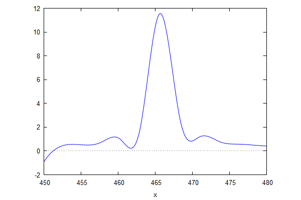
Fig. 1. Frequency of 466.16 Hz.

wxplot2d([discrete, makelist((i-1)*sampleRate/N, i, 170, 180), map(lambda([u], abs(realpart(u))), firstn(rest(transformed, 169),11))]);

Fig. 2. Zooming in a little closer on the points.

So, let's take these same points and try a cubic spline.

load("interpol")$ f: cspline(map(lambda([f,a], [f, a]), makelist((i-1)*sampleRate/N, i, 170, 180), map(lambda([u], abs(realpart(u))), firstn(rest(transformed, 169),11)))); wxplot2d(f, [x, 450, 480]);

Fig. 3. Cubic spline view of things. Still looks fake. But less fake in the middle.

The cubic spline is helpfully printed out with characteristic functions which are mainly readable. I pick out the one that has the interval of concern, namely, 0.5264689995542815*x^3-738.1894409400452*x^2+345013.3968874384*x-5.374983574143041*10^7. We can use differentiation to find the location of the maximum value.

findMax: 0.5264689995542815*x^3-738.1894409400452*x^2+345013.3968874384*x-5.374983574143041*10^7; diff(findMax, x); float(solve(diff(findMax, x)=0, [x]));  

Which gives roots of [x=465.6995765525049,x=469.0682718425062]. Clearly 465.7 is the one we want. We're not any closer than we were last time using linear interpolation, although the general appearance of the graph looks more realistic and we did include another bit of the Maxima library.

FFT - Local Symmetry Inferred Peak

As I was thinking about the previous post, I thought there might be a way to estimate the location of the peak. That is, to find the location in between the discrete data points where the peak probably occurs. 

I tried using realpart and imagpart and abs to see the differences and it seemed like realpart gives me the best view of the relative amplitudes when there are multiple frequencies involved. I also decided to apply an index shift since that seems to match the frequency better although I'm not satisfied with it technically yet.

Let's zoom in on the location of one of the peaks and see what it looks like:

wxplot2d([discrete, makelist((i-1)*sampleRate/N, i, 160, 170), map(lambda([u], abs(realpart(u))), firstn(rest(transformed, 159),11))]);

Fig. 1. Looks like we should be able to make a better guess than just picking one of the points.

Here are the actual points as frequency, absolute, real part value pairs:

[[427.972412109375,1.373307119161833],[430.6640625,1.783783923237471],[433.355712890625,2.525090138349324],[436.04736328125,4.273342049313825],[438.739013671875,13.47741003943344],[441.4306640625,11.94536977902466],[444.122314453125,4.166745114303215],[446.81396484375,2.532438127248608],[449.505615234375,1.822956914133206],[452.197265625,1.426082632315385],[454.888916015625,1.172306075942115]]

For a first crack at it, we might try linear interpolation on the two pairs of points on either side of the gap that contains the peak. Based on the Wikipedia article of the continuous version, we are certainly deviating from the shape of the real thing. Dauntless we press on to see what we get, because maybe we can live with a slight improvement that we know isn't perfect.

So, here we go do linear interpolation and find the line intersection using Maxima.

Line(A, B) := [x, y] . [A[2]-B[2], B[1]-A[1]] = [A[2]-B[2], B[1]-A[1]] . A; float(solve([ Line([436.04736328125,4.273342049313825],[438.739013671875,13.47741003943344]), Line([441.4306640625,11.94536977902466],[444.122314453125,4.166745114303215])], [x, y]));

[[x=439.729058165623,y=16.86285595968834]]

Let's put that point in the middle and see what it looks like:

revised: [[427.972412109375,1.373307119161833],[430.6640625,1.783783923237471],[433.355712890625,2.525090138349324], [436.04736328125,4.273342049313825],[438.739013671875,13.47741003943344], [439.729058165623,16.86285595968834], [441.4306640625,11.94536977902466],[444.122314453125,4.166745114303215], [446.81396484375,2.532438127248608],[449.505615234375,1.822956914133206],[452.197265625,1.426082632315385],[454.888916015625,1.172306075942115]]$ wxplot2d([discrete, revised]); 

Fig. 2. Hmm, closer, but looks kinda fake to me.

Somewhat predictably, this looks as fake as it really is. I think this graph makes it just how clear that linear interpolation is slightly bogus here. Not completely bogus though, it got us closer, right? So, we've ended up on the left side of the true peak which we know should happen exactly at 440 Hz. Why? The slope on the right side of the true peak is further away from the peak and therefore has a lower (absolute) slope value—it is less steep than it would be if it was closer to the peak. This is the weakness of linear interpolating this. We will end up closer to the higher of the two near-peak points than we should.

To get closer, we might want to try a different type of interpolation. Maybe a cubic spline?

FFT in Maxima

Maxima has a basic fast Fourier transform package called fft. Here's are really basic introduction to using it on music data. We define a basic sine wave form with frequency 440 Hz and amplitude 40 as our input and then run fft on it. The interpretation of the results as frequency depends on coordinating together the sample rate, the total number of samples (N), and the sample index (i).

wave(amp, freq, t) := amp*sin(2*float(%pi)*freq*t); sampleRate: 44100.0$ timeStep: 1/sampleRate$ N: 2^14; inputFFT: makelist(wave(40, 440, t*timeStep), t, 1, N)$ transformed: fft(inputFFT)$ wxplot2d([discrete, makelist(i*sampleRate/N, i, 1, 200), firstn(map(lambda([u], abs(u)), transformed), 200)]);

Fig 1. Looks like about 440 Hz

The thing that most threw me for a loop in trying to make sense of the various sources I read was that the x axis needs to be inferred in order to be comprehensible. I wasn't really clear on what that x-axis was. If you dig into the details of the output numbers, you will find the 164th value, has the maximum value. This implies 164 * 44100 / 2^14 = 441 Hz. So, a bit of error has crept into our interpretation of the result because of the discrete nature of the intermediate result. What this means in theory is that there is a theoretical peak that "should" exist somewhat before the 164th index, but because we aren't working with continuous data, we can't see that peak (at the ~163.47th index 😜--or maybe we should be considering it at the 164.47 "index" and subtract 1, interpreting it as zero based, since the peak is probably between the 164th and 165th index).

If we change the function to have two wave forms at different frequencies (340 Hz and 440 Hz), we get both of these in the result:

Fig. 2. wave(20, 340, t*timeStep) + wave(40, 440, t*timeStep)

Next step, in search of the true peak.