Best Fit Circle: find the center using Excel

Finding the center of a best fit circle depends on minimizing the same function we were concerned with in finding the radius, except that we are going to view it as a function of the center instead of as a function of the radius:

where a and b are the x- and y-coordinates, respectively, of the center and r is given by

What we have here is a function of two variables. It looks like three variables until you realize that r is calculated in terms of the other two. So, we can do a three dimensional plot and see what the scoop is. I used Maxima to do this and obtained a very good view of the surface near the best fit center of the points I have been using in all of my investigations of this problem. Here is the 3D plot of SSE(a,b):

What we are most encouraged to see in this graph is that it looks very smooth and it looks like there is exactly one point that is the lowest point. This lowest point is where the SSE function is minimized and constitutes the best center of the circle. (It might be that there are a few local minima somewhat close together that we could see if we zoomed up really tight to the bottom and we are probably happy with any of these as the "answer". Welcome to numerics.)

These formulae can be used in Excel. Designate two cells for each of the values a and b. You don't know what these are, but start with some guesses for these. You will reference these guesses in your Excel formulae. Put your points in consecutive rows after the pattern (x, y, se, R) where se references the x and y for that line as well as the values for a, b, and r. R will only reference x, y for that line and a, b from above. r above is the average of all the R values in the rows (don't include the 1/n in the R)--you may want to create a cell to contain this average and reference it in your se columns. Use absolute references for a, b, and r (if you have a cell for it) so you can copy and paste the formula easily. Make a sum formula at the bottom of your SSE column and it represents your SSE function as above. You want to use the Excel solver now. The SSE cell is the cell you tell it to minimize and the a and b cells you designate as the cells to be modified. The solver will tweak with the a and b values in an attempt to make SSE as small as possible. (The instructions about r and R might seem circular until you actually implement them. Follow through to the end and you'll see it really isn't circular.) Don't try too hard to follow the instructions--try to do the likely intent (as always).

For a Maxima approach see here.

The Polygon Worksheet

I have put together a worksheet in Excel to demonstrate a technique for calculating the vertices of a regular polygon.  You can download the worksheet here.

Overview

It demonstrates an application of vector rotation (and, by the way, complex number multiplication makes a good way to remember how to do vector rotation).  The motivating principle is to demonstrate how you can reduce calls to trigonometric functions while calculating vertices of a regular polygon.  Note that the spreadsheet does not give such (time) savings because it uses both methods: (1) direct calls to trig functions for each vertex in columns B and C and (2) vector rotation in columns E and F.  Also, the error of the vector rotation results is given in columns H and I.  You will notice that the error becomes larger as the vertex number increases.  The error occurs in the vector rotation method, not the trig function method (which is our control, since we believe these results represent the best approximation we can achieve using the floating point precision available in Excel).

The only values you should need to adjust are the number of sides cell, the radius cell, and the initial angle cell.  Everything else follows from these values.  A few notes are in order:

1. The polygon that is determined, is inscribed inside of the circle with the given radius, and centered around the origin. 
2. All angles are specified and calculated in radian measure.
3. If fewer than 50 vertices are needed, the rows will repeat.
4. If you wanted the center somewhere other than the origin, just apply a translation to the points.  So, if you want center (a, b), then each point P = (x, y), becomes P' = (x + a, y + b).  If you've made it this far into this post, you are probably more than capable.

Why Try to Reduce Calls to Trig Functions?

As the user of calculation software and scientific calculators, you may be wondering why we would want to reduce our use of trig functions.  The main reason would be for time-critical applications.  This particular spreadsheet is obviously not one of those, but it demonstrates the accuracy of the method.  So, how do I know that trigonometric functions take a long time to perform.  First of all, let me debunk some myths:

1. Computers and calculators have tables of numbers in them that they use to determine values of "complicated" functions.  So wrong!  Computers and calculators compute/calculate these values!
2. The calculations that computers and calculators do are just based on tables and interpolation.  This is rarely true.  Sometimes a programmer will use a method like this when he knows that the precision needs of his application will be met this way and will be much faster.  But it is actually more programming effort and would only be done when you didn't need very accurate results but you needed them really, really fast.
3. Computers and calculators have hardware circuits that make the complex calculations almost as fast as the simple ones.  Not so.  Fact:  Multiplication is done with the fmult instruction.  Addition is done with the fadd instruction.  fmult takes way, way more computer cycles to compute than fadd.  fsincos takes way, way longer than fmult.  It is an unavoidable consequence of the nature of these calculations.

Recall that multiplication is dependant on addition.  Several additions actually.  So it should come as no surprise that by the time you put together a circuit that does the job that several additions and small multiplications can do, you end up with a circuit that takes longer to complete than one that just does addition.

The same is true of trig functions.  You know how you calculate them?  Here are the magic formulas:

The dots (...) indicate that it goes on and on and on and on and on, until the changes are small enough that you aren't changing the digits that mater to you. You may need more terms than are listed to get the accuracy you need. These formulas above are not written in the most computationally efficient manner, but you can rest assured that any circuitry or coding or combination thereof, which computes the values of the above functions will take longer than 4 multiplications and 2 addition/subtractions will (those are the operations involved in doing vector rotation).

Enter Vector Rotation

The key to how this method helps us, is that we can use a few trig function calls at the beginning and reuse the results several times over. We compute the direction vector for the central angle, θ, that each side covers. For a hexagon, this angle is 360°/6 = 60°, or π/3.

We need to determine the value of the central angle using direct calls to trig functions, but we will be able to reuse those values.  We also call trig functions to get our initial position.  From there we use our vector rotation method.  So, E14 and F14 use the values in E11 and F11 (renamed mx and my) and those of E13 and F13 to find their values:

E14 =E13*mx-F13*my

F14 =E13*my+F13*mx

Cells in rows below 14 do the same thing.  They still reference mx and my, which are the cosine and sine of our central angle, θ, respectively, and they reference the cells directly above them.  The concept for each row is:  rotate the point in the row above me around the origin by the central angle and tell me the x and y values for that rotated point.

Proof of the Formulas

Suppose we are given a point (x, y) and denote the distance from the origin as r and the angle it makes with the positive axis as i.  We wish to rotate (x, y) counter-clockwise about the origin by angle θ.  The diagram below illustrates:

Our new point (x', y') can be simplified:

                  

                      
                      
                 
                     
                     

If you look back at the formulas for E14 and F14, you may observe that mx and my correspond with sin θ and cos θ and E13 and F13 correspond with x and y.  That's all there is to it. 

Relationship with Complex Number Multiplication

If we represent the new point (x', y') as x' + y'j (where j is used to indicate the square root of -1), we can say:

This will produce an equivalent result to what we have above.

Best Fit Circle: find radius given center

Given a center (a, b) of a circle, we want to find the best fit radius, r, to a set of given points P_i = (x_i , y_i), for i = 1 to n. By addressing the relationship between best radius for a given set of points, we will be able to make r dependent on a and b, rather than being something we guess at independently. (This is ground work for another post.)

In other words, we have a set of points and a candidate center for what we think is a good approximation to a circle (or a circular arc). We want to find the best radius for that center with those points and have a means of quantifying how good of a fit we have. If we can find this, we can decide which of a set of candidate centers is best.

The usual thing to do when looking for a best fit shape is to minimize the sum of squares of the errors. If we knew the radius we might calculate the sum of squares of the errors as

So, for each point, we find out how far it is from the candidate center, find the difference between that distance and the radius to get the error, and then square the error. And then we add all of those squared errors together to get SSE(r). We want to minimize SSE(r), which is a simple problem in differential calculus. When SSE’(r) = 0, SSE(r) is at a minimum, maximum, or perhaps a point of inflection. Then

Observe that the best fit radius is just the average distance from the candidate center to each point. Seems sensible. Also, observe that

and so, by the second derivative test, SSE(r) is at a minimum.

To see it all put together into a practical solution, see Best Fit Circle: find the center using Excel.

Field Measurement of Circular Arcs

There are a number of simple cases for field measurement of a circle. A full circle can be measured across its diameter or around its circumference to determine its area. (To use the circumference to determine the area, first use the formula C = 2πr to determine the radius and then use the radius to determine the area which gives A = C²/(4π).) Half circles and quarter circles are similarly straightforward.

But suppose you want to measure a circular arc which has an unknown central angle, θ, such that 0 < θ < 180°. There are three things that are normally easy to measure for such circles and they only require a tape measure:

1. 1. chord distance (also called the run of the arc – denoted u)
2. 2. rise of the arc (i)
3. 3. arc length (s) – arc length measurements are easy for existing items if there is a (normally vertical) surface to hold the tape against; not as easy for proposed items unless approximation is acceptable

The following diagram illustrates:

There are number of reasons why you might be interested in the rise, run approach to defining a circular arc. If you are laying out an arc, it may be infeasible to run a tape measure around the center point of the arc – perhaps due to the size or interfering objects. Also, measuring unusual angles requires specialized equipment (such as a transit) which requires set up time. (If you are using a total station this whole discussion is moot, so we are assuming we’re trying to do something without it.) The rise/run approach is also the approach used in some blue prints for defining curved walls. Carpenters and linear measurements are on good working terms, and we like to leverage this where we can.

But whatever the reason you might want to use this approach, you can calculate both ways. First of all, let’s list all of the relevant equations:

 (1)

 (2)

                     

 (3)

         

(4)

Now, let’s suppose we know u and i. We determine the remaining variables from these.
Manipulating equation (4):

(5)

So, we need a and θ (or at least cos θ) to find r, which we do by manipulating equations (1) and (3).
Manipulating equation (3):

(6)

Manipulating equation (1):

(7)

Substitute (6) and (7) into equation (5):

(8)

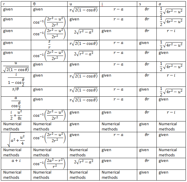
Now that we have r we can use that number in equation (7) to find θ, etc. I omit all of the rest of the gory details, but here are the final results for solving the unknowns in terms of different combinations of known values (note that θ is understood to be in radian measure and the reader is left to discern what order to calculate the different values in).

I have not addressed how to solve the cases where s and either u, i, or a are given as they are more difficult.  Perhaps a future post will address these cases.

Field Measurement of Quadrilaterals Using Only a Tape Measure

Trapezoids

A common nonrectangular area that needs to me measured in the field is a trapezoid. Sometimes shapes are approximated by a trapezoid, if a rectangle is not considered a reasonable approximation or not easily visualized. The well-known formula for the area of a trapezoid is

                        

where b₁ and b₂ are the lengths of the two parallel sides and h is the distance between them (measured perpendicularly to the parallel sides, of course). It is noteworthy that the (b₁+b₂)/2 can be interpreted as the average of the lengths of the parallel sides. This is the length of a line referred to as the median of the trapezoid. In the field, it is often more convenient/faster to measure the median and the height (h, also called the altitude) than to measure both bases and the height. If the location of the median can be “eye-balled” with sufficient precision for the purposes being met, this may increase productivity by decreasing the number of measurements needed. For more information on the trapezoid and the median, see a description here.

General Case Quadrilateral

There are (at least) two approaches to measuring the area quadrilaterals when nothing is known about the internal angles or “parallelness” of nonadjacent lines. The following diagram displays both methods.

We can determine the area of this shape by making 5 measurements and produce an exact picture, or by taking 3 measurements and getting an approximate area. Both are “area by triangles” methods.

Area by Triangles – Heron Method

If we measure the sides AB, BC, CD, DA, and one of the diagonals (either AC or BD), we can use Heron’s theorem to determine the area of the triangles on either side of the chosen diagonal. We can use the law of cosines and law of sines to determine the angles. Alternatively, a basic AutoCAD drawing using temporary construction-line circles would allow you to determine these results without manual calculations. This would give us a full description of the area. This method also generalizes well to an arbitrary number of sides (but requiring a lot of measurements--don't use this method).

Area by Triangles – By Altitude

On the other hand, we could measure the length of a diagonal (say, AC), leave the measuring tape in place (or replace with a string line) and use a second tape measure to measure from the other vertices (B and D) to the diagonal. As long as the accuracy/precision of the result desired is not too high, we can “eye-ball” perpendicular to the diagonal to get the heights of the triangles to an acceptable accuracy. The area calculation is obvious from there. This method involves fewer measurements, minimal extra equipment, and is quicker to calculate, which may make it more efficient for a quadrilateral. It does not generalize to an n-sided figure as easily as the previous method, but could be done with additional string lines used simultaneously.

Introducing the Twisted Plane

This idea is motivated by something that comes up often in the world of surveying. Not always do we have simple straight lines, and not always do we have a simple plane. Here is an example of the situation in plan view:

You may know that three points define a plane and that an arbitrary fourth point, may not be on the same plane. We can unambiguously define the elevation of every point on the outside of our rectangle by "stringing a line" (which is surveyor-speak for straight interpolation). We want the elevations we would get if we pulled a string really tight all the way around the outside of the rectangle. (If you care about the units, call them meters, but they are not really the point of this example.)

What about arbitrary points on the interior of the rectangle?  It is possible to use interpolation schemes to determine the elevation of a point on the interior of a plane such that it will coincide with the plane. But in the above situation, we have four points that are not coplanar.  A common, and highly adaptable, solution to this problem is to break our region up into triangles.  There are two ways we could do this.

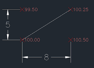
Case 1

Notice that in case 1 the elevation at the midpoint of the diagonal line would be 100.125 m.

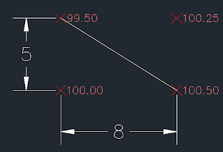
Case 2

On the other hand, the elevation at the middle of the diagonal line drawn in case 2 would be 100.000 m.

The general case of this sort of procedure - breaking a region up into triangles - is called creating a triangular irregular network (TIN) and is a well established method.  The fact that there may be multiple solutions which are not equivalent does not normally concern us.  We just pick one that works because all we care about is that the water will run.  In a complex plan, it is not uncommon to see the choice of lines given on the plan.  As a surveyor you like to see that as it mean the ambiguity of your job is largely removed.

When it comes to disadvantages, the first thing that is noteworthy about the TIN is that triangles and graders (or their operators) do not like each other very much. Although the grader is a very versatile machine, it still likes following a line. Rectangles are ideal. Look up at case 2 and pretend you're driving a grader, starting from the SW corner and proceeding to the SE corner. As you approach the SE corner, you have a problem: you've got two edges that you are trying to put the blade against. This is frankly infeasible. If this is a very large area (5 miles by 8 miles), we don't care, because the tricky spot is so small compared with the total area.  For a smaller area, this might be significant. So what happens? The watchword is "blend", which basically means the grader operator is supposed to figure it out himself and "make it work."

So, can we model this "blending"? (I don't mean just at the diagonal edge, I want to get rid of that.) Can we figure out what the math looks like that describes the result which the grader (operator) would produce if given four corner points on a small, rectangular area and told to "blend" and "make it work"? If we can do this, then we can apply this same method to areas too big for the grader to cover in just one or two passes. Or apply it to the problem of setting grades on concrete islands that are on such a surface. I call it a twisted plane and it allows us to completely discard the diagonal line.

A twisted plane is a surface formed by using a line (segment) and "sweeping" laterally while changing its angle. The line segment is just like the blade of a grader running from one edge of the rectangle to the opposite side. If the width of our rectangle was exactly the width of the grader blade, it would begin with north end of the blade at elevation 99.50 m and the south end at 100.00 m at the west edge of the area. As the grader proceeded to the east the blade would gradually change its angle from having 0.500 m fall from south to north to having 0.250 m fall from the south to north. (The realities of grading are somewhat swept under the carpet for the sake of simplicity.) Here is an attempt to show what the terrain would look like:

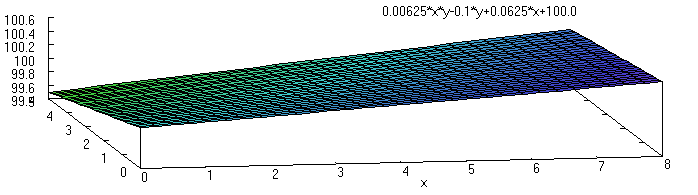
GNU plot of "twisted plane" performed using Maxima

We will now proceed to develop the equation which describes this surface.  Let's start with a fresh diagram that uses variables in it:

For completeness, here are the equations for the elevations of the north, south, east, and west line elevations (we take the south-west corner as the origin):

Now, to determine the elevation at any point on the interior, we can use the west and east lines and do straight interpolation across them like so:

This produces the equation:

If we were to use the north and south lines and interpolate across them instead, we would get:

In both cases the resulting equation is