Equation of Circle in 3D and Snap Tangent

For a time I was on a bit of an AutoCAD like calculation kick and went through some interesting calculations like snap tangent, snap perpendicular, and intersection of a line with a plane. I wanted to take the next step on snap tangent and consider snap tangent to a sphere.

Snap tangent means, start with some point and try to find a point on the destination object (circle, sphere, ellipse, anything) that causes the line segment between the first point and the second point to be tangent to the object selected. My post about snap tangent, showed the result for a circle and worked in 2D. If you get the concept in 2D and are ready to take the concept to 3D for a sphere, you probably recognize without proof that the set of possible points on the sphere which will result in a tangential point, forms a circle. You can pretty much mentally extrapolate from the following picture which a repeat from the previous post.

Fig. 1 - Can you imagine the snap tangent circle on this if we allow the figure to represent a sphere? The snap tangent circle has center \(E\) and radius \(a\).

I will not repeat the method of calculation from the previous post but will simply observe that we can produce the values \(E\) and \(a\), which are the center and radius of the snap tangent circle. We add to this the normal of this circle, \(N = A - C\), and then normalize \(N\).

So, now we need a way to describe this circle which is not too onerous. A parametric vector equation is the simplest expression of it. We take our inspiration from the classic representation of circles in parametric form, which is
\[ p(\theta) = (x(\theta), y(\theta)) \] \[ x(\theta) = r \cos{\theta} \] \[ y(\theta) = r \sin{\theta}. \]
We have a normal from which to work from, but we need to have an entire coordinate system to work with. The classic parametric equations have everything in a neat coordinate system, but to describe a circle that's oriented any which way, we need to cook up a coordinate system to describe it with. Observe a change to the foregoing presentation that we can make:
\[ p(\theta) = r \cos{\theta} (1, 0) + r \sin{\theta} (0, 1) = r \cos{\theta} \vec{x} + r \sin{\theta} \vec{y}\]
The normal vector we have is basically the z-axis of the impromptu coordinate system we require, but we don't have a natural x-axis or y-axis. The trouble is there are an infinite number of x-axes that we could choose, we just need something perpendicular to \(N = (n_x, n_y, n_z).\) So, let's just pick one. If I take the cross product between \(N\) and any other vector that isn't parallel to \(N\), I will obtain a value which is perpendicular to \(N\) and it can serve as my impromptu x-axis. To ensure I don't have a vector which is close to the direction of \(N\), I will grab the basis vector, which is the most "out of line" with the direction of \(N\). So, for example (F# style),

        let b = if abs(normal.[0]) <= abs(normal.[1]) then    
                    if abs(normal.[0]) <= abs(normal.[2]) then
                        DenseVector([| 1.0; 0.0; 0.0 |])
                    else
                        DenseVector([| 0.0; 0.0; 1.0 |])
                else
                    if abs(normal.[1]) <= abs(normal.[2]) then
                        DenseVector([| 0.0; 1.0; 0.0 |])
                    else
                        DenseVector([| 0.0; 0.0; 1.0 |])

In this case, I have 

\[\vec{x} = b \times N\] \[\vec{y} = N \times \vec{x}.\]

Using this impromptu coordinate system, I can express an arbitrary circle in parametric form, having center \(C\) and radius \(r\) as

\[ p(\theta) = C + \vec{x} r \cos{\theta} + \vec{y} r \sin{\theta}.\]

Thus, our snap tangent circle is given from above as 

\[ p(\theta) = E + \vec{x} a \cos{\theta} + \vec{y} a \sin{\theta},\]

where we would use \(N = A - C\) (normalized) to be the beginning of our coordinate system.

Circle Fitting in Maxima

In previous posts, I've considered the problem of fitting a circle to 2D data points. Fitting problems such as this require:

1. An equation form to fit to. 
2. A function to quantify the error, which is to be minimized.

For a circle, the form of equation we want to fit to is
\[r^2=(x-a)^2 + (y-b)^2.\]
Maxima's lsquares package removes the burden of item number 2 for us. But for interest's sake, the error function we want to minimize can be given as

\[\mathrm{r}\left( a,b\right) =\frac{\sum_{i=1}^{n}\sqrt{{\left( {x}_{i}-a\right) }^{2}+{\left( {y}_{i}-b\right) }^{2}}}{n}\]

\[\mathrm{SSE}\left( a,b\right) =\sum_{i=1}^{n}{\left( \mathrm{r}\left( a,b\right) -\sqrt{{\left( {x}_{i}-a\right) }^{2}+{\left( {y}_{i}-b\right) }^{2}}\right) }^{2}.\]

Recalling that \(\sum_{i=1}^{n}(\bar{x}-x_i)^2 = \sum_{i=1}^{n}{x_i}^2 - (\sum_{i=1}^{n}{x_i})/n\), we see that
\[\mathrm{SSE}\left( a,b\right) =\sum_{i=1}^{n}\left({\left( {x}_{i}-a\right) }^{2}+{\left( {y}_{i}-b\right) }^{2}\right)-\frac{{\left(\sum_{i=1}^{n}\sqrt{{\left({x}_{i}-a\right) }^{2}+{\left( {y}_{i}-b\right) }^{2}}\right)}^{2}}{n}.\]

lsquares_estimates()

Given a set of points in matrix form (m), we need only to use the equation of a circle and indicate which are the data point variables and which are the "solve for" variables. In our problem,

lsquares_estimates(m, [x,y], (x-a)^2 + (y-b)^2 = r^2, [a,b,r]);

will suffice. The following function can be used to check the SSE.

sse(a, b, r, pts) := sum((r-sqrt((pts[i][1]-a)^2+(pts[i][2]-b)^2))^2,i,1,length(pts));

Testing for Reasonableness

It is reasonable to ask whether least squares (or other data fitting methods) will reliably produce good results with a particular quality of data for a particular application. This is true for any problem. What if the math works fine, but the likelihood of being able to "math filter" the  likely errors in the data to reach an accurate answer is not so high? In other words, how much inaccuracy in the collected data can you tolerate and still have a reasonable expectation of getting to the right answer? I'm not going to attempt to deal with probabilities (per se) or confidence intervals, but look at a simulation approach that may be able to give you an idea of the reasonableness of the circle fit based on an (intuitively) estimated amount of random error in your data.

Simulation of Circular Arc Data

We will consider the problem of data collected, using a total station, of a circular arc, with an "as-built" scenario particularly in view. As such, auto-generated sample points should simulate the expected behaviors of a rod/prism person stepping out regular sample locations from start to end of an ostensibly circular arc. This can be implemented as random normal perturbations of a circular arc.

One of the first pieces to a realistic perturbed circle is to be able to apply randomization that follows a normal distribution given an expected value and a standard deviation. Maxima has a function that behaves this way. random_normal() can be called with an expected value and standard deviation and optionally with a number of values to generate. Here is a sample use and output of the function, pictured using the histogram function:

load(distrib)$
load(draw)$

histogram(

    random_normal(50.0, 1.0, 1000),

    nclasses = 10,

    xrange = [40,60]);

Fig. 1. Normally distributed data

The standard deviation should be chosen such that roughly two-thirds of the time (≈68%), the sample value will be within one standard deviation of the mean; that is, on the interval \((\bar{x}-\sigma, \bar{x}+\sigma).\) 

Where the radius is concerned, we have the relatively predictable variations of the prism person's actions and the relatively unpredictable variations of the ostensible circular arc, which could turn out to not be an arc at all. In the absence of any sort of meaningful solution to this latter variation, we could possibly just bump up the standard deviation. But I'm not clear on whether this is a meaningful thing to do in assessing the acceptability of the data collection precision. The error should be "small" if the thing we measured conforms well to a circle. In order to check for whether this is "small" you need to produce a standard deviation from the SSE: \[\sigma_{SSE} = \sqrt{\frac{SSE}{n-1}}\] In the scenario we're dealing with here, someone would probably draw the computed arc in a CAD program and compare it to the measured data points and in an "arm-waving" sort of way decide whether it looks good or not.

Where the point sampling distances are concerned, we will assume that the rod person can step out distances (or angle sweeps) within some percentage of that intended. We will also make the pragmatic assumption that the prism person has decided a definite number of samples per given arc and will try to make them evenly spaced. The prism person will try to subdivide the remaining space at each sample point, and two thirds of the time, they will be within some percentage of the distance (or angle sweep) they intended.

Here is the perturbedArc() function with a sample usage:

perturbedArc(angle, center, radius, probable_radius_error, sample_spacing_variability, number_points) := block( [initAngle, termAngle, radii, expectedSweep, actualSweep, angles, remainingAngle, i], initAngle: random(float(2*%pi)), termAngle: float(initAngle + angle), remainingAngle: float(angle), angles: [initAngle, termAngle], radii: random_normal(radius, probable_radius_error, number_points), for i: (number_points-1) thru 2 step -1 do ( expectedSweep: remainingAngle/i, actualSweep: random_normal(expectedSweep, sample_spacing_variability*expectedSweep), remainingAngle: remainingAngle - actualSweep, angles: cons(termAngle - remainingAngle, angles) ), angles: sort(angles), map(lambda([r,theta],bfloat(center+r*[cos(theta),sin(theta)])), radii, angles) )$ pts: perturbedArc(1.5*%pi, [1000,1000], 3000, 12, 0.05, 20)$ wxplot2d([discrete,pts], [style,points], [same_xy,true]);

Fig. 2 - This is a perturbed circular arc. Doesn't look very perturbed does it? If we bumped up the standard deviation of the radius enough, we'd get something more clearly perturbed.

To produce the matrix form of the data I use a simple function I created (see here) called MakeMatrix(). Beyond that, it is a simple as

m: MakeMatrix(pts)$
lsquares_estimates(m, [x,y], (x-a)^2 + (y-b)^2 = r^2, [a,b,r]);
subst(%[1],sse(a,b,abs(r),pts));

Best Fit Circle: find the center using Excel

Finding the center of a best fit circle depends on minimizing the same function we were concerned with in finding the radius, except that we are going to view it as a function of the center instead of as a function of the radius:

where a and b are the x- and y-coordinates, respectively, of the center and r is given by

What we have here is a function of two variables. It looks like three variables until you realize that r is calculated in terms of the other two. So, we can do a three dimensional plot and see what the scoop is. I used Maxima to do this and obtained a very good view of the surface near the best fit center of the points I have been using in all of my investigations of this problem. Here is the 3D plot of SSE(a,b):

What we are most encouraged to see in this graph is that it looks very smooth and it looks like there is exactly one point that is the lowest point. This lowest point is where the SSE function is minimized and constitutes the best center of the circle. (It might be that there are a few local minima somewhat close together that we could see if we zoomed up really tight to the bottom and we are probably happy with any of these as the "answer". Welcome to numerics.)

These formulae can be used in Excel. Designate two cells for each of the values a and b. You don't know what these are, but start with some guesses for these. You will reference these guesses in your Excel formulae. Put your points in consecutive rows after the pattern (x, y, se, R) where se references the x and y for that line as well as the values for a, b, and r. R will only reference x, y for that line and a, b from above. r above is the average of all the R values in the rows (don't include the 1/n in the R)--you may want to create a cell to contain this average and reference it in your se columns. Use absolute references for a, b, and r (if you have a cell for it) so you can copy and paste the formula easily. Make a sum formula at the bottom of your SSE column and it represents your SSE function as above. You want to use the Excel solver now. The SSE cell is the cell you tell it to minimize and the a and b cells you designate as the cells to be modified. The solver will tweak with the a and b values in an attempt to make SSE as small as possible. (The instructions about r and R might seem circular until you actually implement them. Follow through to the end and you'll see it really isn't circular.) Don't try too hard to follow the instructions--try to do the likely intent (as always).

For a Maxima approach see here.

Best Fit Circle: find radius given center

Given a center (a, b) of a circle, we want to find the best fit radius, r, to a set of given points P_i = (x_i , y_i), for i = 1 to n. By addressing the relationship between best radius for a given set of points, we will be able to make r dependent on a and b, rather than being something we guess at independently. (This is ground work for another post.)

In other words, we have a set of points and a candidate center for what we think is a good approximation to a circle (or a circular arc). We want to find the best radius for that center with those points and have a means of quantifying how good of a fit we have. If we can find this, we can decide which of a set of candidate centers is best.

The usual thing to do when looking for a best fit shape is to minimize the sum of squares of the errors. If we knew the radius we might calculate the sum of squares of the errors as

So, for each point, we find out how far it is from the candidate center, find the difference between that distance and the radius to get the error, and then square the error. And then we add all of those squared errors together to get SSE(r). We want to minimize SSE(r), which is a simple problem in differential calculus. When SSE’(r) = 0, SSE(r) is at a minimum, maximum, or perhaps a point of inflection. Then

Observe that the best fit radius is just the average distance from the candidate center to each point. Seems sensible. Also, observe that

and so, by the second derivative test, SSE(r) is at a minimum.

To see it all put together into a practical solution, see Best Fit Circle: find the center using Excel.

Field Measurement of Circular Arcs

There are a number of simple cases for field measurement of a circle. A full circle can be measured across its diameter or around its circumference to determine its area. (To use the circumference to determine the area, first use the formula C = 2πr to determine the radius and then use the radius to determine the area which gives A = C²/(4π).) Half circles and quarter circles are similarly straightforward.

But suppose you want to measure a circular arc which has an unknown central angle, θ, such that 0 < θ < 180°. There are three things that are normally easy to measure for such circles and they only require a tape measure:

1. 1. chord distance (also called the run of the arc – denoted u)
2. 2. rise of the arc (i)
3. 3. arc length (s) – arc length measurements are easy for existing items if there is a (normally vertical) surface to hold the tape against; not as easy for proposed items unless approximation is acceptable

The following diagram illustrates:

There are number of reasons why you might be interested in the rise, run approach to defining a circular arc. If you are laying out an arc, it may be infeasible to run a tape measure around the center point of the arc – perhaps due to the size or interfering objects. Also, measuring unusual angles requires specialized equipment (such as a transit) which requires set up time. (If you are using a total station this whole discussion is moot, so we are assuming we’re trying to do something without it.) The rise/run approach is also the approach used in some blue prints for defining curved walls. Carpenters and linear measurements are on good working terms, and we like to leverage this where we can.

But whatever the reason you might want to use this approach, you can calculate both ways. First of all, let’s list all of the relevant equations:

 (1)

 (2)

                     

 (3)

         

(4)

Now, let’s suppose we know u and i. We determine the remaining variables from these.
Manipulating equation (4):

(5)

So, we need a and θ (or at least cos θ) to find r, which we do by manipulating equations (1) and (3).
Manipulating equation (3):

(6)

Manipulating equation (1):

(7)

Substitute (6) and (7) into equation (5):

(8)

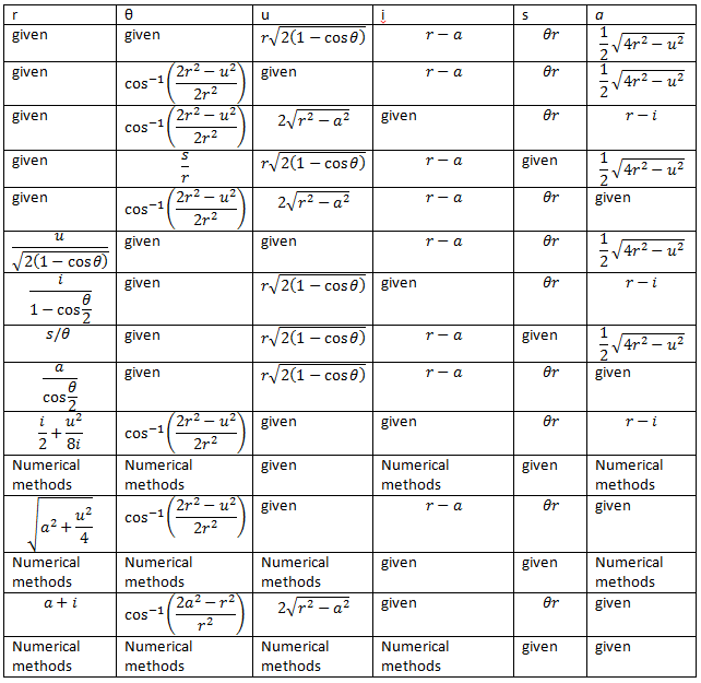
Now that we have r we can use that number in equation (7) to find θ, etc. I omit all of the rest of the gory details, but here are the final results for solving the unknowns in terms of different combinations of known values (note that θ is understood to be in radian measure and the reader is left to discern what order to calculate the different values in).

I have not addressed how to solve the cases where s and either u, i, or a are given as they are more difficult.  Perhaps a future post will address these cases.